Deep Reinforcement Learning
Introduction
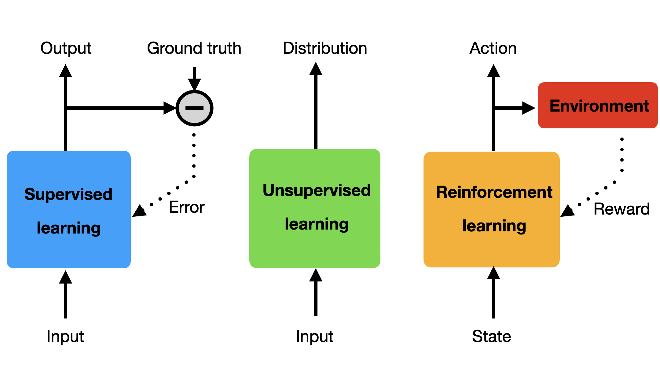
Different types of machine learning depending on the feedback
Supervised learning: the correct answer (ground truth) is provided to the algorithm, the prediction error drives learning directly.
Unsupervised learning: no answer is given to the system, the learning algorithm extracts a statistical model from raw inputs.
Reinforcement learning: an estimation of the correctness of the answer is provided by the environment through the reward function.
The RL bible


Sutton and Barto (1998) . Reinforcement Learning: An Introduction. MIT Press.
Sutton and Barto (2017) . Reinforcement Learning: An Introduction. MIT Press. 2nd edition.
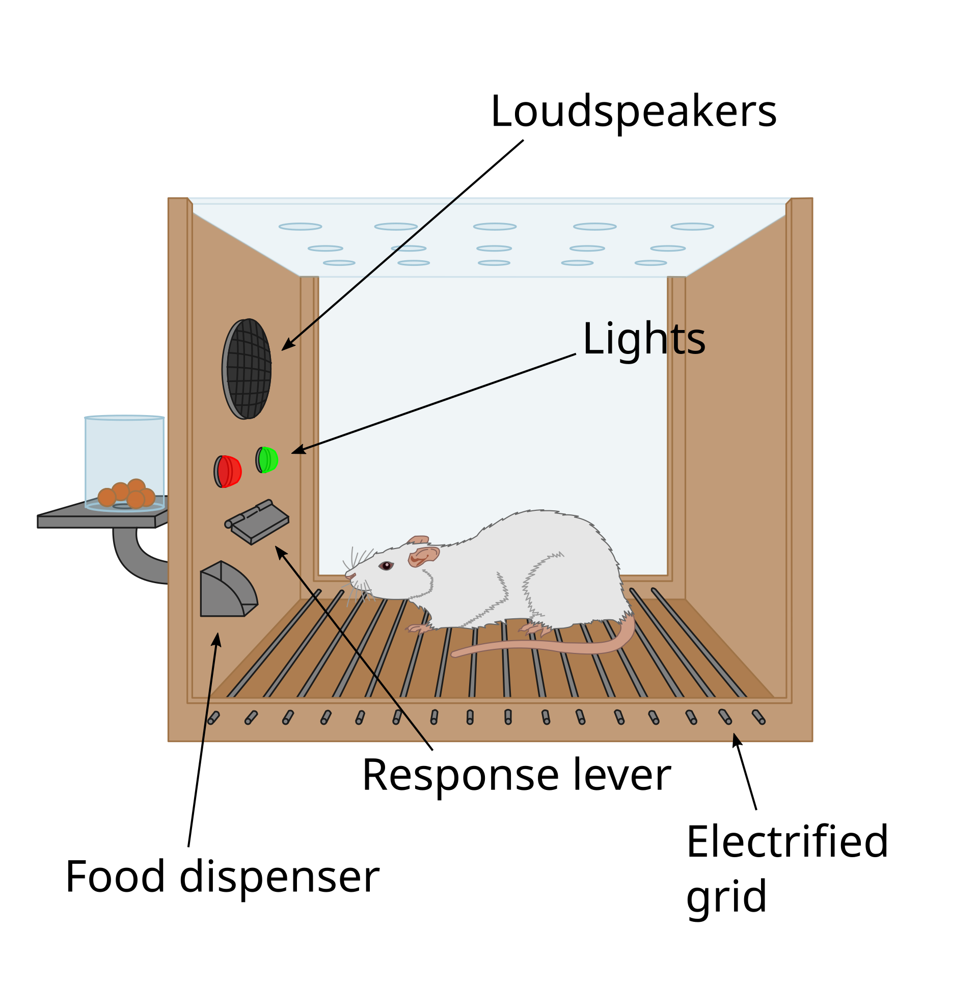
Operant conditioning
Reinforcement learning comes from animal behavior studies, especially operant conditioning / instrumental learning.
Thorndike’s Law of Effect (1874–1949) suggested that behaviors followed by satisfying consequences tend to be repeated and those that produce unpleasant consequences are less likely to be repeated.
Positive reinforcements (rewards) or negative reinforcements (punishments) can be used to modify behavior (Skinner’s box, 1936).
This form of learning applies to all animals, including humans:
Training (animals, children…)
Addiction, economics, gambling, psychological manipulation…
Behaviorism: only behavior matters, not mental states.
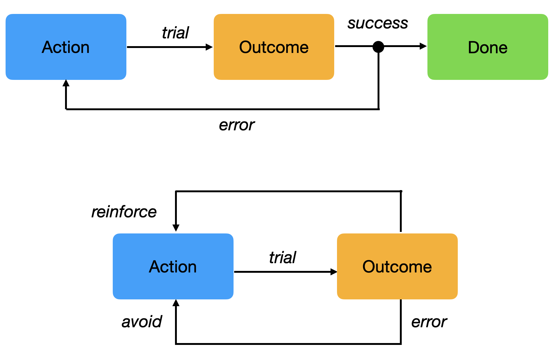
Trial and error learning
The key concept of RL is trial and error learning: trying actions until the outcome is good.
The agent (rat, robot, algorithm) tries out an action and observes the outcome.
If the outcome is positive (reward), the action is reinforced (more likely to occur again).
If the outcome is negative (punishment), the action will be avoided.
After enough interactions, the agent has learned which action to perform in a given situation.
Trial and error learning
The agent has to explore its environment via trial-and-error in order to gain knowledge.
The agent’s behavior is roughly divided into two phases:
The exploration phase, where it gathers knowledge about its environment.
The exploitation phase, where this knowledge is used to collect as many rewards as possible.
The biggest issue with this approach is that exploring large action spaces might necessitate a lot of trials (sample complexity).
The modern techniques we will see in this course try to reduce the sample complexity.

The agent-environment interface
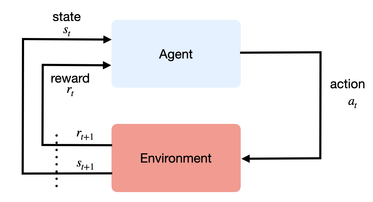
The agent and the environment interact at discrete time steps: t=0, 1, …
The agent observes its state at time t: s_t \in \mathcal{S}
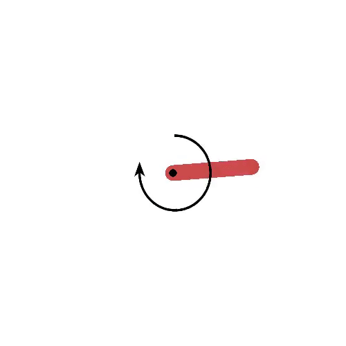
It produces an action at time t, depending on the available actions in the current state: a_t \in \mathcal{A}(s_t)
It receives a reward according to this action at time t+1: r_{t+1} \in \Re
It updates its state: s_{t+1} \in \mathcal{S}
- The behavior of the agent is therefore is a sequence of state-action-reward-state (s, a, r, s') transitions.
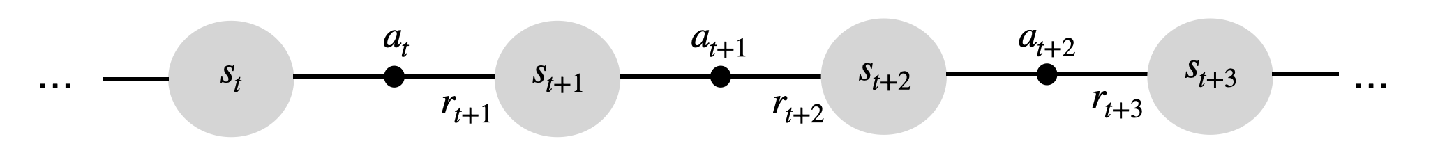
- Sequences \tau = (s_0, a_0, r_1, s_1, a_1, \ldots, s_T) are called episodes, trajectories, histories or rollouts.
The agent-environment interface
Environment and agent states
The state s_t can relate to:
the environment state, i.e. all information external to the agent (position of objects, other agents, etc).
the internal state, information about the agent itself (needs, joint positions, etc).
Generally, the state represents all the information necessary to solve the task.
The agent generally has no access to the states directly, but to observations o_t:
o_t = f(s_t)
Example: camera inputs do not contain all the necessary information such as the agent’s position.
Imperfect information define partially observable problems.
Policy
What we search in RL is the optimal policy: which action a should the agent perform in a state s?
The policy \pi maps states into actions.
- It is defined as a probability distribution over states and actions:
\begin{aligned} \pi &: \mathcal{S} \times \mathcal{A} \rightarrow P(\mathcal{S})\\ & (s, a) \rightarrow \pi(s, a) = P(a_t = a | s_t = s) \\ \end{aligned}
- \pi(s, a) is the probability of selecting the action a in s. We have of course:
\sum_{a \in \mathcal{A}(s)} \pi(s, a) = 1
- Policies can be probabilistic / stochastic. Deterministic policies select a single action a^*in s:
\pi(s, a) = \begin{cases} 1 \; \text{if} \; a = a^* \\ 0 \; \text{if} \; a \neq a^* \\ \end{cases}
Reward function
The only teaching signal in RL is the reward function.
The reward is a scalar value r_{t+1} provided to the system after each transition (s_t,a_t, s_{t+1}).
Rewards can also be probabilistic (casino).
The mathematical expectation of these rewards defines the expected reward of a transition:
r(s, a, s') = \mathbb{E}_t [r_{t+1} | s_t = s, a_t = a, s_{t+1} = s']
Rewards can be:
dense: a non-zero value is provided after each time step (easy).
sparse: non-zero rewards are given very seldom (difficult).
Returns
The goal of the agent is to find a policy that maximizes the sum of future rewards at each timestep.
The discounted sum of future rewards is called the return:
R_t = \sum_{k=0}^\infty \gamma ^k \, r_{t+k+1}
Rewards can be delayed w.r.t to an action: we care about all future rewards to select an action, not only the immediate ones.
Example: in chess, the first moves are as important as the last ones in order to win, but they do not receive reward.
Supervised learning
Correct input/output samples are provided by a superviser (training set).
Learning is driven by prediction errors, the difference between the prediction and the target.
Feedback is instantaneous: the target is immediately known.
Time does not matter: training samples are randomly sampled from the training set.
Reinforcement learning
Behavior is acquired through trial and error, no supervision.
Reinforcements (rewards or punishments) change the probability of selecting particular actions.
Feedback is delayed: which action caused the reward? Credit assignment.
Time matters: as behavior gets better, the observed data changes.
Optimal control
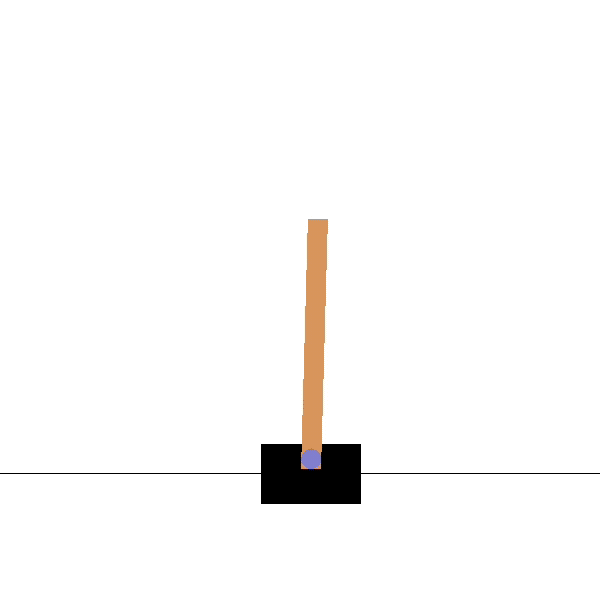
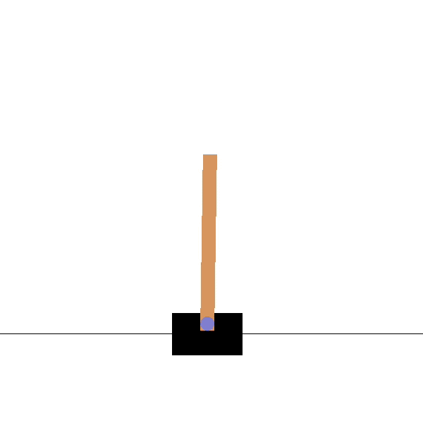
Pendulum
Goal: maintaining the pendulum vertical.

States: angle and velocity of the pendulum.
Actions: left and right torques.
Rewards: cosine distance to the vertical.
Optimal control
Cartpole
Goal: maintaining the pole vertical by moving the cart left or right.
States: position and speed of the cart, angle and velocity of the pole.
Actions: left and right movements.
Rewards: +1 for each step until failure.
Board games (Backgammon, Chess, Go, etc)
TD-Gammon (Tesauro, 1992) was one of the first AI to beat human experts at a complex game, Backgammon.
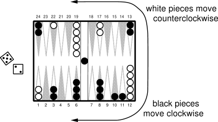
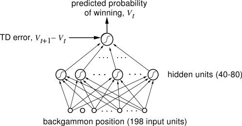
States: board configurations.
Actions: piece displacements.
Rewards: +1 for game won, -1 for game lost, 0 otherwise. sparse rewards
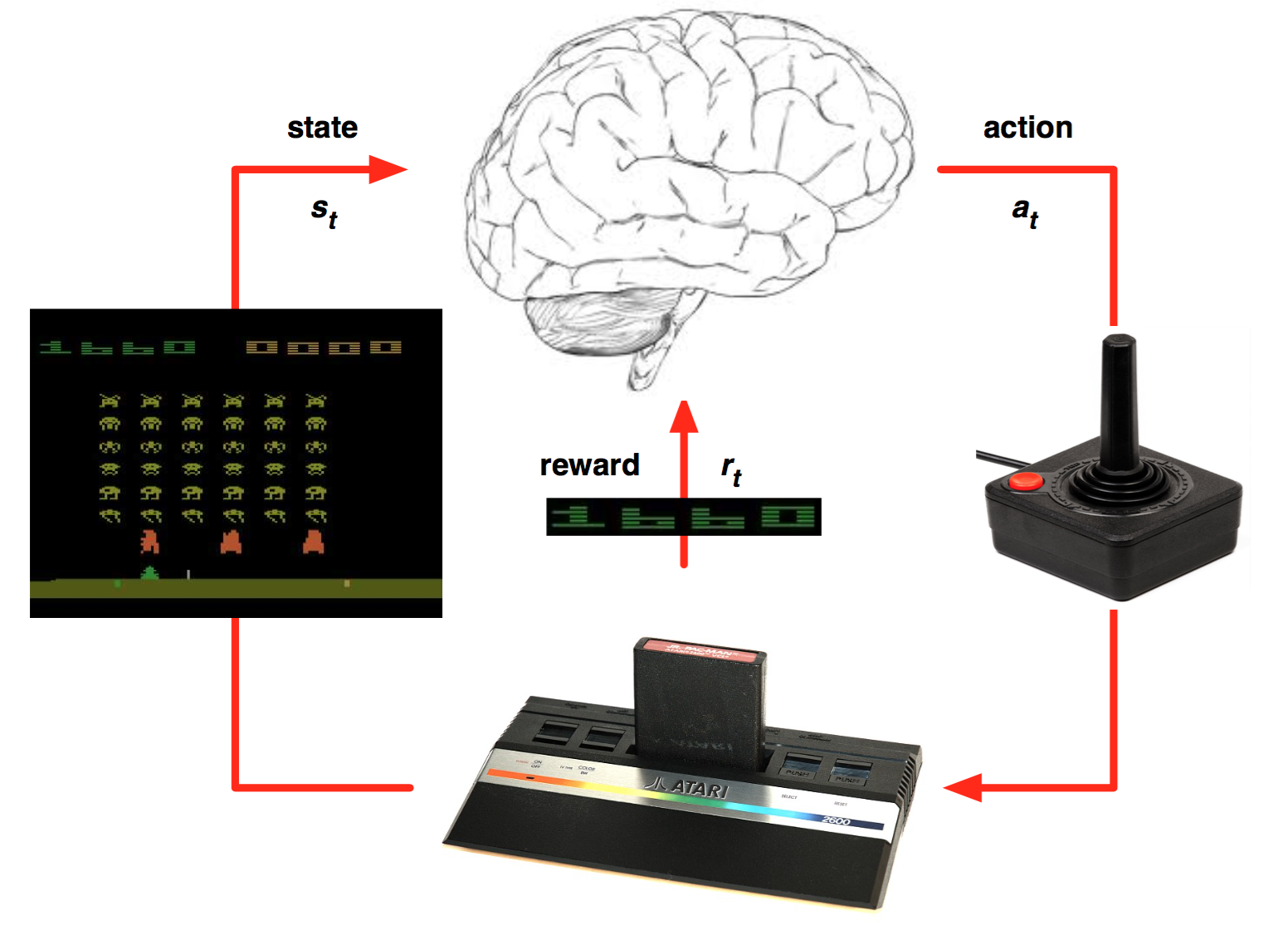
Deep Reinforcement Learning (DRL)
Classical tabular RL was limited to toy problems, with few states and actions.
It is only when coupled with deep neural networks that interesting applications of RL became possible.
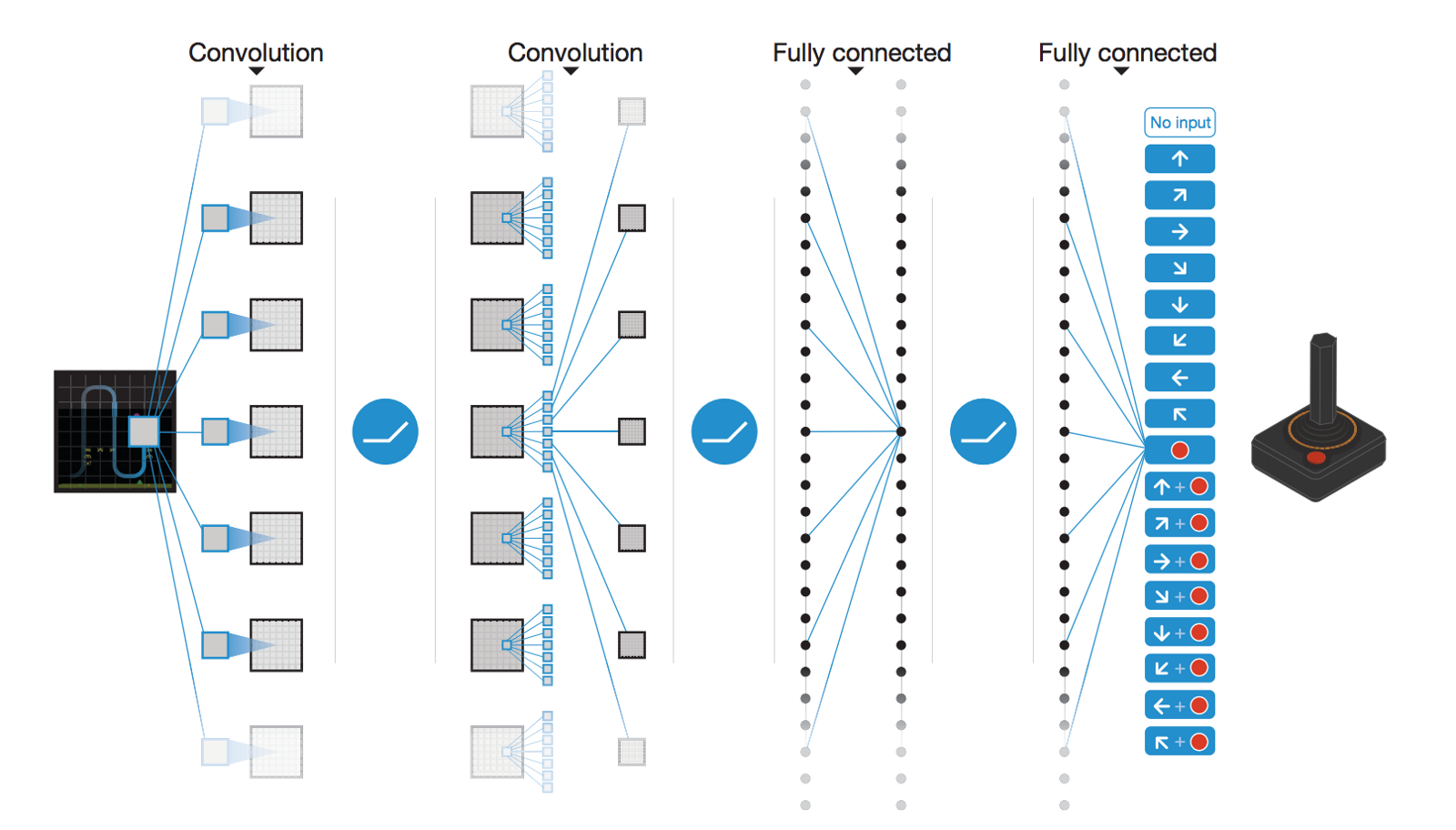
Deepmind (now Google) started the deep RL hype in 2013 by learning to solve 50+ Atari games with a CNN.
AlphaGo
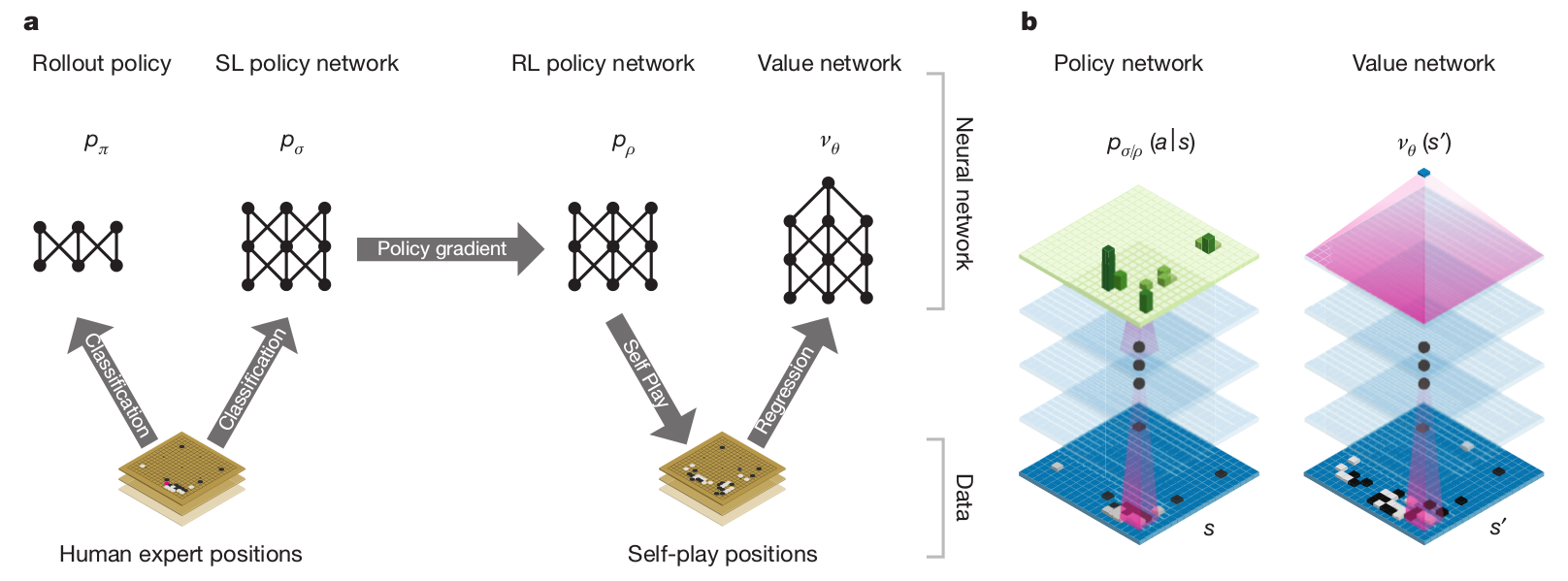
AlphaGo was able to beat Lee Sedol in 2016, 19 times World champion.
It relies on human knowledge to bootstrap a RL agent (supervised learning).
The RL agent discovers new strategies by using self-play: during the games against Lee Sedol, it was able to use novel moves which were never played before and surprised its opponent.
Training took several weeks on 1202 CPUs and 176 GPUs.
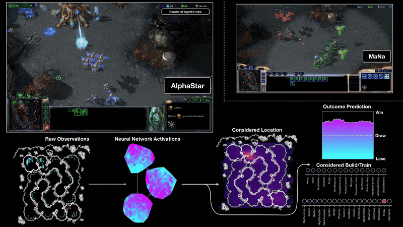
Starcraft II (AlphaStar)
Process control

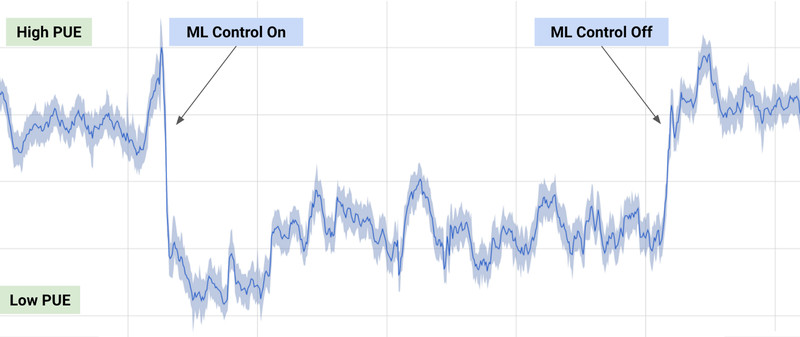
40% reduction of energy consumption when using deep RL to control the cooling of Google’s datacenters.
States: sensors (temperature, pump speeds).
Actions: 120 output variables (fans, windows).
Rewards: decrease in energy consumption
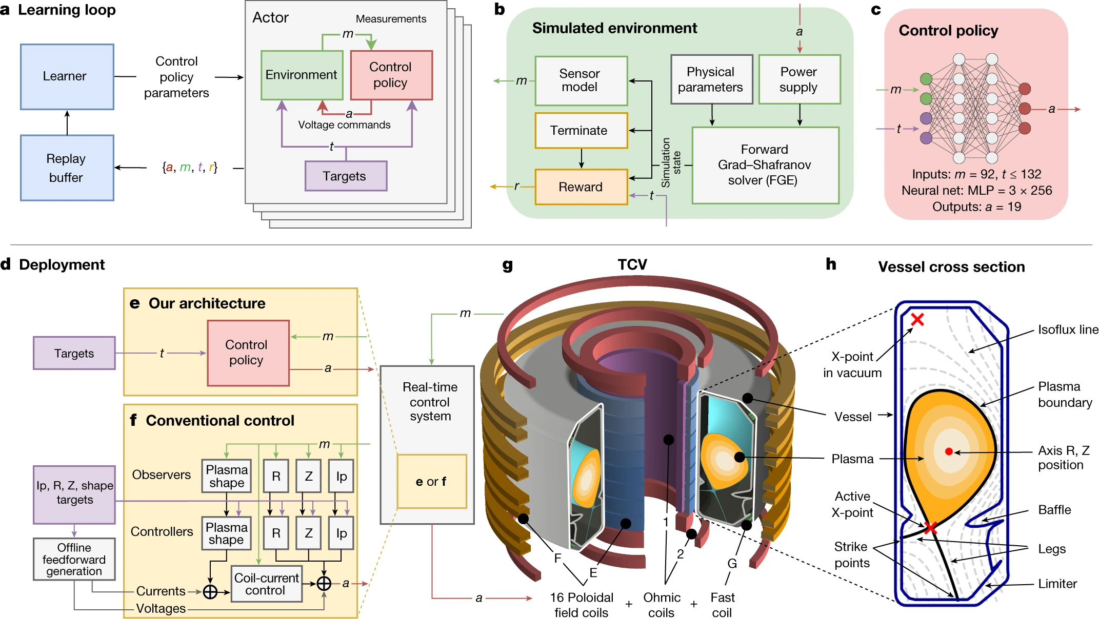
Magnetic control of tokamak plasmas
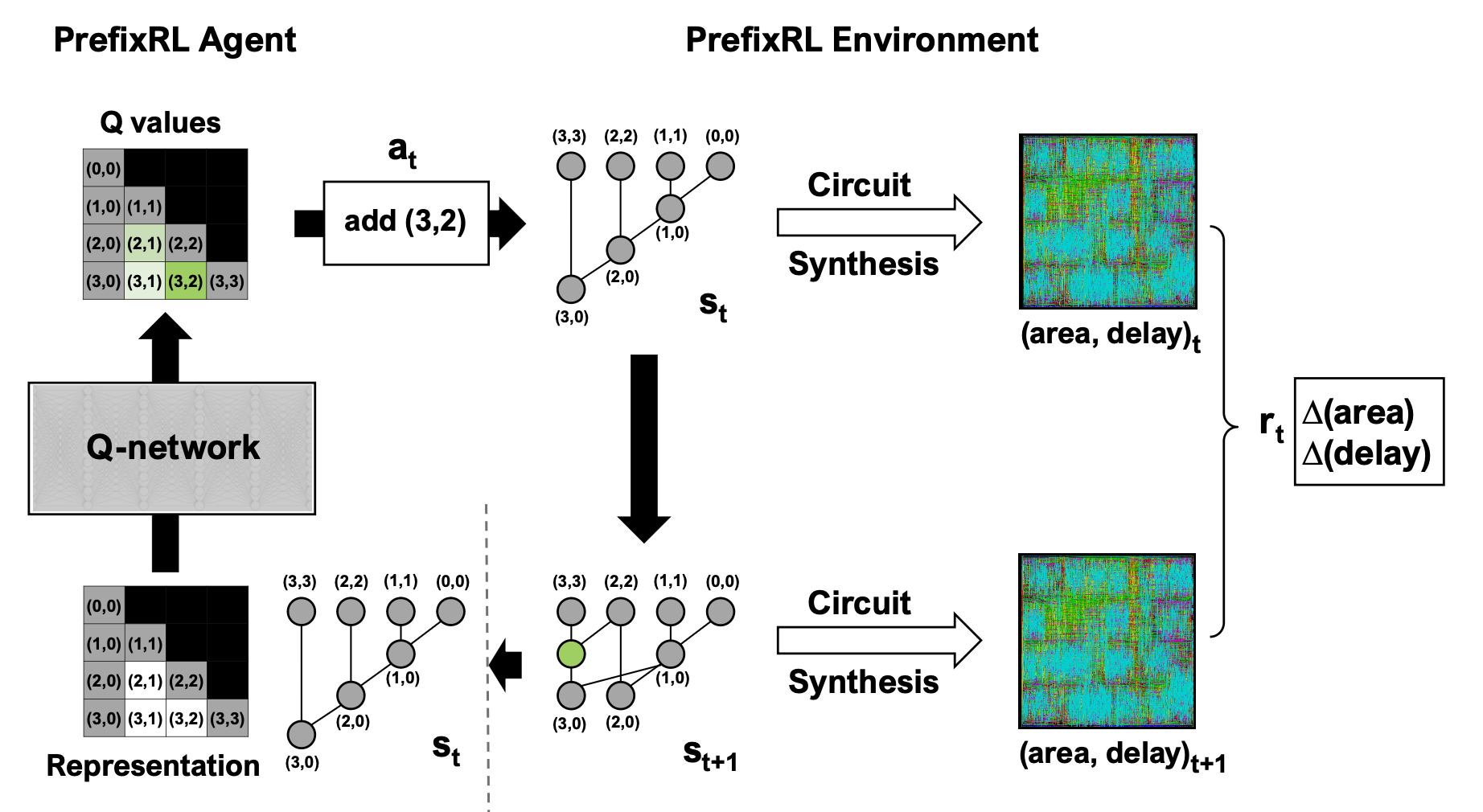
Chip design
ChatGPT
