Deep Reinforcement Learning

Deep Q-Learning

Julien Vitay

Professur für Künstliche Intelligenz - Fakultät für Informatik

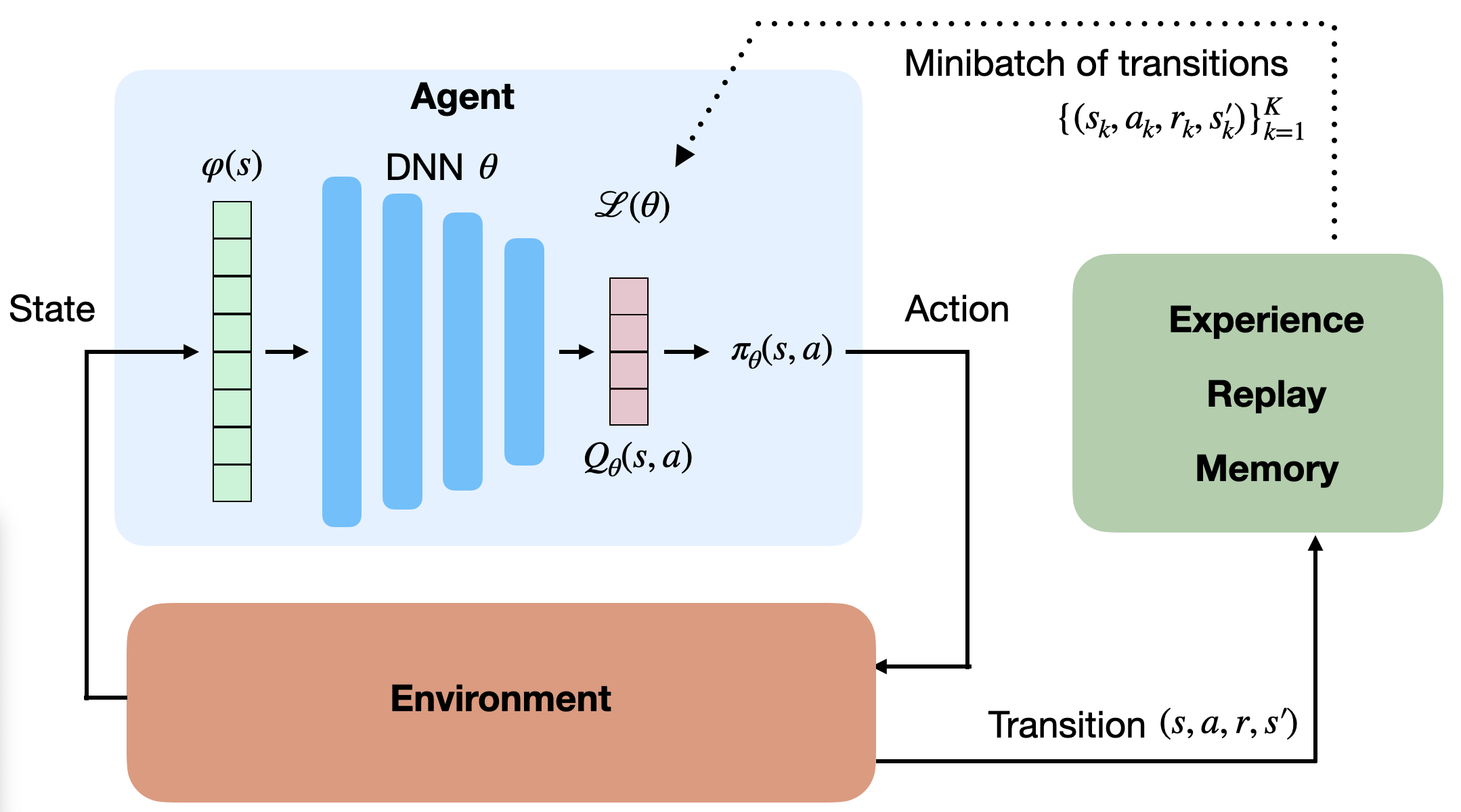
Value-based deep RL

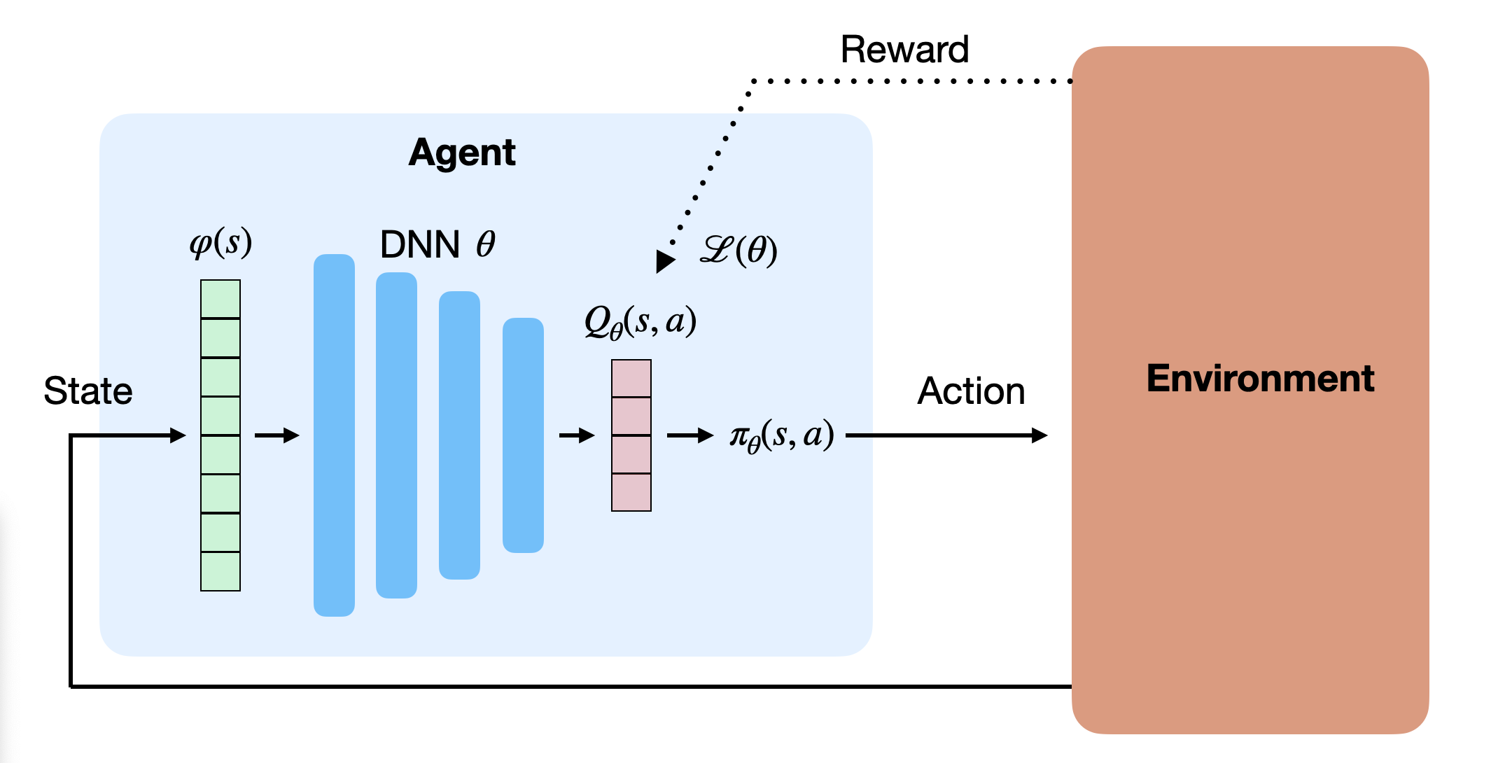
• The basic idea in value-based deep RL is to approximate the Q-values in each possible state, using a deep neural network with free parameters \theta:

Q_\theta(s, a) \approx Q^\pi(s, a) = \mathbb{E}_\pi (R_t | s_t=s, a_t=a)

• The Q-values now depend on the parameters \theta of the DNN.

• The derived policy \pi_\theta uses for example an \epsilon-greedy or softmax action selection scheme over the estimated Q-values:

\pi_\theta(s, a) \leftarrow \text{Softmax} (Q_\theta(s, a))

Function approximators to learn the Q-values

There are two possibilities to approximate Q-values Q_\theta(s, a):

• The DNN approximates the Q-value of a single (s, a) pair.

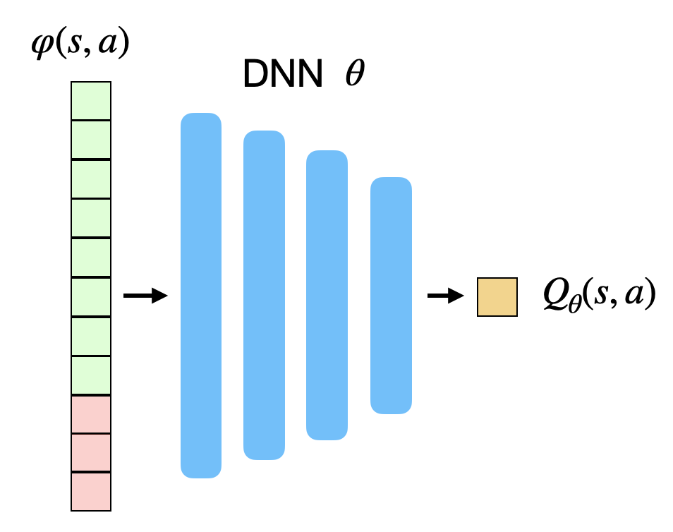
• The action space can be continuous.

• The DNN approximates the Q-value of all actions a in a state s.

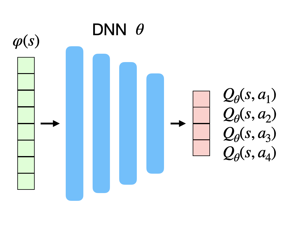
• The action space must be discrete (one neuron per action).

First naive approach: Q-learning with function approximation

We could simply adapt Q-learning with FA to the DNN:

• Initialize the deep neural network with parameters \theta.

• Start from an initial state s_0.

• for t \in [0, T_\text{total}]:

  • Select a_{t} using a softmax over the Q-values Q_\theta(s_t, a).

  • Take a_t, observe r_{t+1} and s_{t+1}.

  • Update the parameters \theta by minimizing the loss function:

  \mathcal{L}(\theta) = (r_{t+1} + \gamma \, \max_{a'} Q_\theta(s_{t+1}, a') - Q_\theta(s_t, a_t))^2

  • if s_t is terminal: sample another initial state s_0.

Remark: We will now omit the break for terminal states, it is always implicitly here.

DNN need stochastic gradient descent

• This naive approach will not work: DNNs cannot learn from single examples (online learning = instability).

• DNNs require stochastic gradient descent (SGD):

\mathcal{L}(\theta) = E_\mathcal{D} (||\textbf{t} - \textbf{y}||^2) \approx \frac{1}{K} \sum_{i=1}^K ||\textbf{t}_i - \textbf{y}_i||^2

• The loss function is estimated by sampling a minibatch of K i.i.d samples from the training set to compute the loss function and update the parameters \theta.

• This is necessary to avoid local minima of the loss function.

• Although Q-learning can learn from single transitions, it is not possible using DNN.

• Why not using the last K transitions to train the network? We could store them in a transition buffer and train the network on it.

Second naive approach: Q-learning with a transition buffer

• Initialize the deep neural network with parameters \theta.

• Initialize an empty transition buffer \mathcal{D} of size K: \{(s_k, a_k, r_k, s'_k)\}_{k=1}^K.

• for t \in [0, T_\text{total}]:

  • Select a_{t} using a softmax over the Q-values Q_\theta(s_t, a).

  • Take a_t, observe r_{t+1} and s_{t+1}.

  • Store (s_t, a_t, r_{t+1}, s_{t+1}) in the transition buffer.

  • Every K steps:

    • Update the parameters \theta using the transition buffer:

    \mathcal{L}(\theta) = \frac{1}{K} \, \sum_{k=1}^K (r_k + \gamma \, \max_{a'} Q_\theta(s'_k, a') - Q_\theta(s_k, a_k))^2

    • Empty the transition buffer.

Correlated inputs

• Unfortunately, this does not work either.

• The last K transitions (s, a, r, s') are not i.i.d (independent and identically distributed).

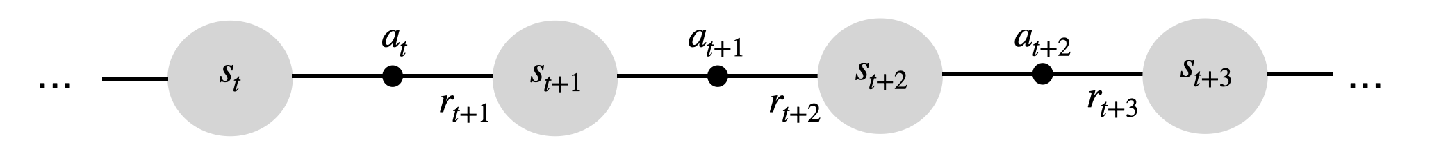
• The transition (s_{t+1}, a_{t+1}, r_{t+2}, s_{t+2}) depends on (s_{t}, a_{t}, r_{t+1}, s_{t+1}) by definition, i.e. the transitions are correlated.

• Even worse, when playing video games, successive frames will be very similar or even identical.

• The actions are also correlated: you move the paddle to the left for several successive steps.

Correlated inputs

• Feeding transitions sequentially to a DNN is the same as giving all MNIST 0’s to a DNN, then all 1’s, etc… It does not work.

• In SL, we have all the training data before training: it is possible to get i.i.d samples by shuffling the training set between two epochs.

• In RL, we create the “training set” (transitions) during training: the samples are not i.i.d as we act sequentially over time.

Non-stationarity

• In SL, the targets \mathbf{t} do not change over time: an image of a cat stays an image of a cat throughout learning.

\mathcal{L}(\theta) = \mathbb{E}_{\mathbf{x}, \mathbf{t} \sim \mathcal{D}} [||\mathbf{t} - F_\theta(\mathbf{x})||^2]

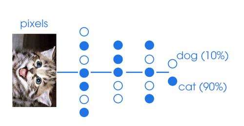
• The problem is said stationary, as the distribution of the data does not change over time.

Non-stationarity

• In RL, the targets t = r + \gamma \, \max_{a'} Q_\theta(s', a') do change over time:

  • Q_\theta(s', a') depends on \theta, so after one optimization step, all targets have changed!

  • As we improve the policy over training, we collect higher returns.

\mathcal{L}(\theta) = \mathbb{E}_{s, a \sim \pi_\theta} [(r + \gamma \, \max_{a'} Q_\theta(s', a') - Q_\theta(s, a))^2]

• NN do not like this. After a while, they give up and settle on a suboptimal policy.

Illustration of non-stationary targets

• We want our value estimates to “catch” the true values.

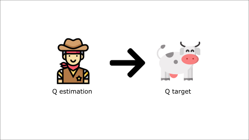
Illustration of non-stationary targets

• We update our estimate to come closer to the target.

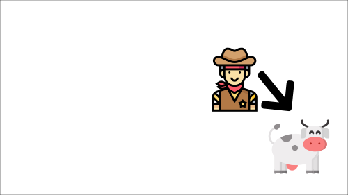
Illustration of non-stationary targets

• But the target moves! We need to update again.

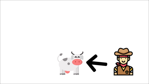
Illustration of non-stationary targets

• This leads to very strange and inefficient optimization paths.

1 - Deep Q-networks (DQN)

Problem with non-linear approximators and RL

• Non-linear approximators never really worked with RL before 2013 because of:

  1. The correlation between successive inputs or outputs.

  2. The non-stationarity of the problem.

• These two problems are very bad for deep networks, which end up overfitting the learned episodes or not learning anything at all.

• Deepmind researchers proposed to use two classical ML tricks to overcome these problems:

  1. experience replay memory.

  2. target networks.

Experience replay memory

• To avoid correlation between samples, (Mnih et al. 2015) proposed to store the (s, a, r, s') transitions in a huge experience replay memory or replay buffer \mathcal{D} (e.g. 1 million transitions).

• When the buffer is full, we simply overwrite old transitions.

• The Q-learning update is only applied on a random minibatch of those past experiences, not the last transitions.

• This ensure the independence of the samples (non-correlated samples).

Experience replay memory

• Initialize value network Q_{\theta}.

• Initialize experience replay memory \mathcal{D} of maximal size N.

• for t \in [0, T_\text{total}]:

  • Select an action a_t based on Q_\theta(s_t, a), observe s_{t+1} and r_{t+1}.

  • Store (s_t, a_t, r_{t+1}, s_{t+1}) in the experience replay memory.

  • Every T_\text{train} steps:

    • Sample a minibatch \mathcal{D}_s randomly from \mathcal{D}.

    • For each transition (s_k, a_k, r_k, s'_k) in the minibatch:

      • Compute the target value t_k = r_k + \gamma \, \max_{a'} Q_{\theta}(s'_k, a')

    • Update the value network Q_{\theta} on \mathcal{D}_s to minimize:

    \mathcal{L}(\theta) = \mathbb{E}_{\mathcal{D}_s}[(t_k - Q_\theta(s_k, a_k))^2]

Experience replay memory

• But wait! The samples of the minibatch are still not i.i.d, as they are not identically distributed:

  • Some samples were generated with a very old policy \pi_{\theta_0}.

  • Some samples have been generated recently by the current policy \pi_\theta.

• The samples of the minibatch do not come from the same distribution, so this should not work.

Experience replay memory

• This should not work, except if you use an off-policy algorithm, such as Q-learning!

Q^\pi(s, a) = \mathbb{E}_{s_t \sim \rho_b, a_t \sim b}[ r_{t+1} + \gamma \, \max_a Q^\pi(s_{t+1}, a) | s_t = s, a_t=a]

• In Q-learning, you can take samples from any behavior policy b, as long as the coverage assumption stands:

\pi(s,a) > 0 \Rightarrow b(s,a) > 0

• Here, the behavior policy b is a kind of “superset” of all past policies \pi used to fill the ERM, so it “covers” the current policy.

b = \{\pi_{\theta_0}, \pi_{\theta_1}, \ldots, \pi_{\theta_t}\}

• Samples from b are i.i.d, so Q-learning is going to work.

• Note: it is not possible to use an experience replay memory with on-policy algorithms.

  Q^\pi(s, a) = \mathbb{E}_{s_t \sim \rho_\pi, a_t \sim \pi}[ r_{t+1} + \gamma \, Q^\pi(s_{t+1}, a_{t+1}) | s_t = s, a_t=a]

  • a_{t+1} \sim \pi_\theta would not be the same between \pi_{\theta_0} (which generated the sample) and \pi_{\theta_t} (the current policy).

Target network

• The second problem when using DNN for RL is that the target is non-stationary, i.e. it changes over time: as the network becomes better, the Q-values have to increase.

• In DQN, the target for the update is not computed from the current deep network \theta:

r + \gamma \, \max_{a'} Q_\theta(s', a')

but from a target network \theta´ updated only every few thousands of iterations.

r + \gamma \, \max_{a'} Q_{\theta'}(s', a')

• \theta' is simply a copy of \theta from the past.

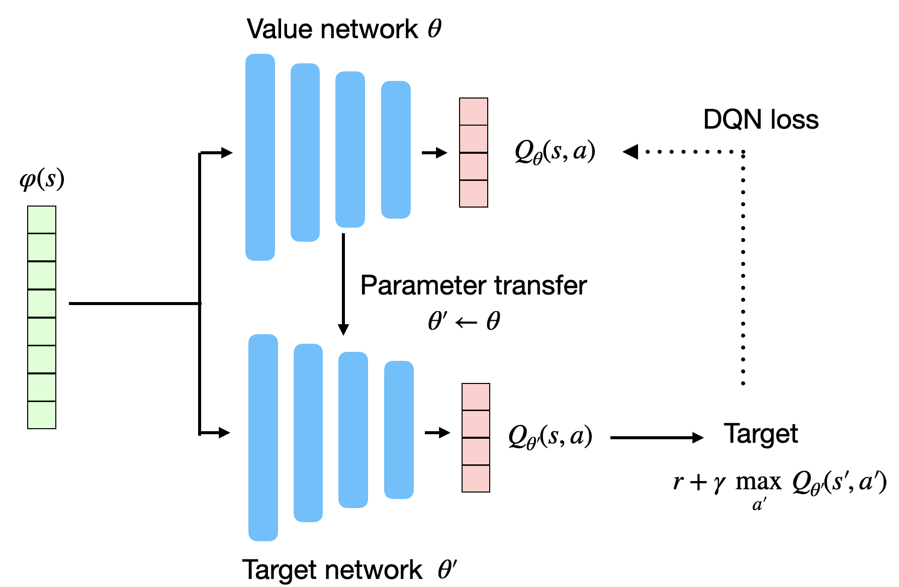
• DQN loss function:

\mathcal{L}(\theta) = \mathbb{E}_\mathcal{D} [(r + \gamma \, \max_{a'} Q_{\theta'}(s', a')) - Q_\theta(s, a))^2]

Target network

• This allows the target r + \gamma \, \max_{a'} Q_{\theta'}(s', a') to be stationary between two updates.

• It leaves time for the trained network to catch up with the targets.

• The update is simply replacing the parameters \theta' with the trained parameters \theta:

\theta' \leftarrow \theta

• The value network \theta basically learns using an older version of itself…

DQN: Deep Q-network

• Initialize value network Q_{\theta} and target network Q_{\theta'}.

• Initialize experience replay memory \mathcal{D} of maximal size N.

• for t \in [0, T_\text{total}]:

  • Select an action a_t based on Q_\theta(s_t, a), observe s_{t+1} and r_{t+1}.

  • Store (s_t, a_t, r_{t+1}, s_{t+1}) in the experience replay memory.

  • Every T_\text{train} steps:

    • Sample a minibatch \mathcal{D}_s randomly from \mathcal{D}.

    • For each transition (s_k, a_k, r_k, s'_k) in the minibatch:

      • Compute the target value t_k = r_k + \gamma \, \max_{a'} Q_{\theta'}(s'_k, a') using the target network.

    • Update the value network Q_{\theta} on \mathcal{D}_s to minimize:

    \mathcal{L}(\theta) = \mathbb{E}_{\mathcal{D}_s}[(t_k - Q_\theta(s_k, a_k))^2]

  • Every T_\text{target} steps:

    • Update target network: \theta' \leftarrow \theta.

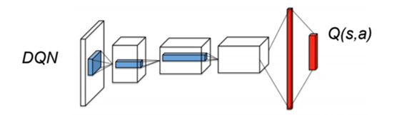
DQN: Deep Q-network

• The deep network can be anything. Deep RL is only about defining the loss function adequately.

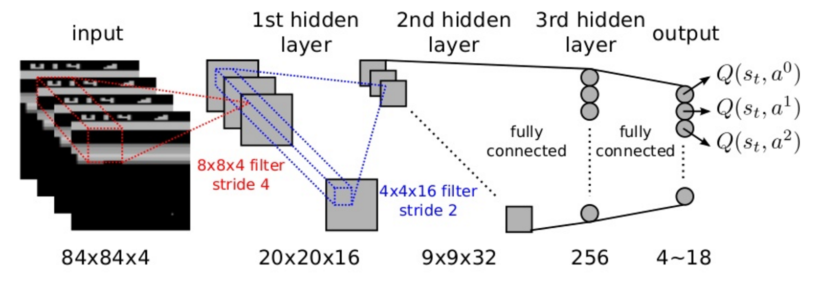
• For pixel-based problems (e.g. video games), convolutional neural networks (without max-pooling) are the weapon of choice.

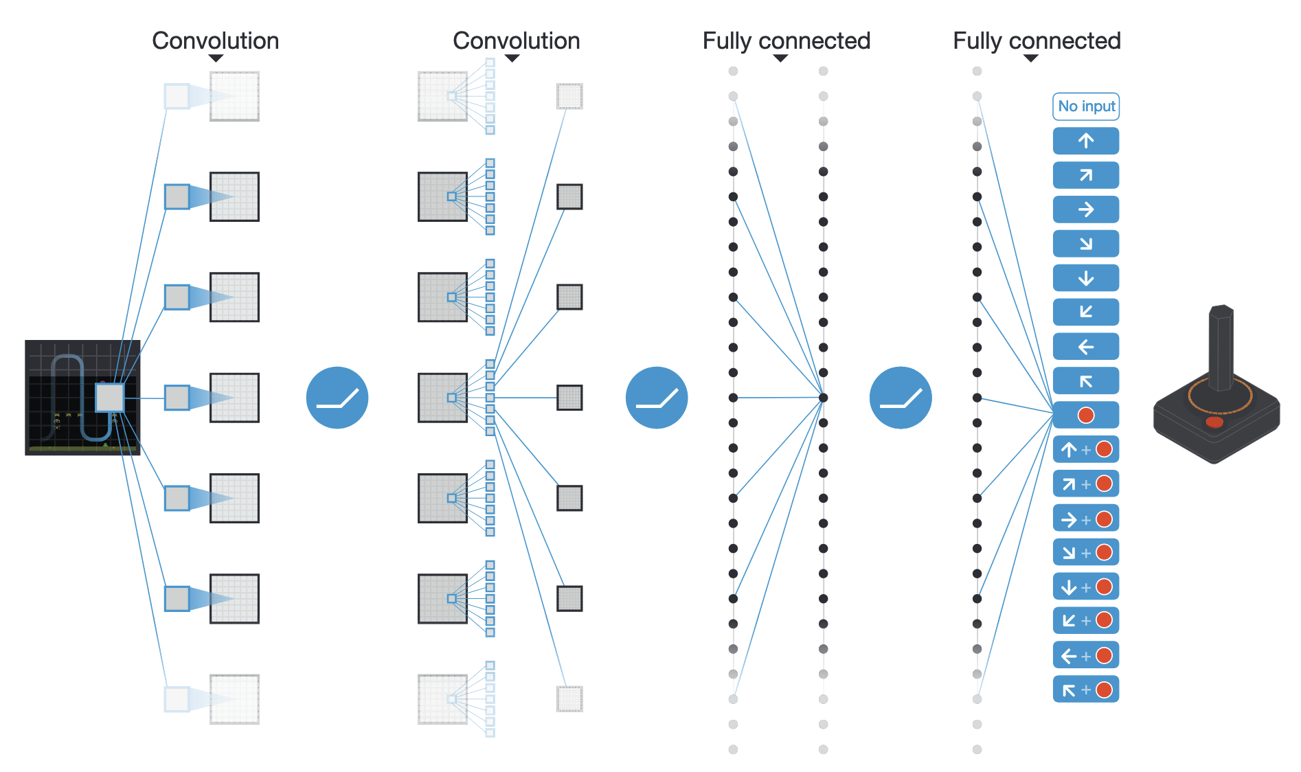
Why no max-pooling?

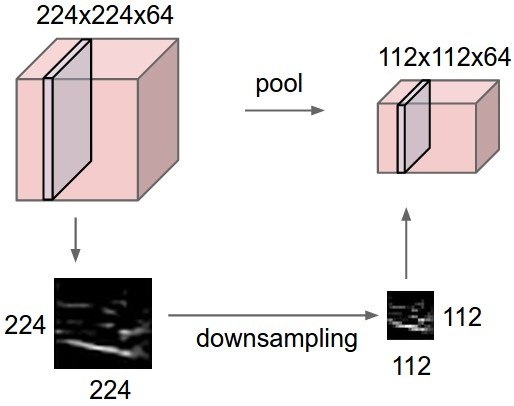
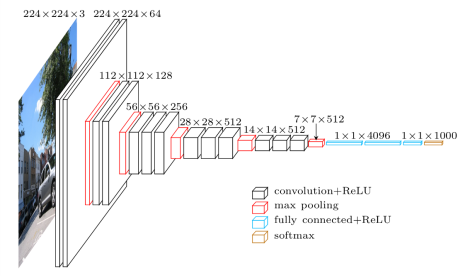
• The goal of max-pooling is to get rid of the spatial information in the image.

• For object recognition, you do not care whether the object is in the center or on the side of the image.

• Max-pooling brings spatial invariance.

• In video games, you want to keep the spatial information: the optimal action depends on where the ball is relative to the paddle.

Are individual frames good representations of states?

• Is the ball moving from the child to the baseball player, or the other way around?

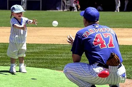
• Using video frames as states breaks the Markov property: the speed and direction of the ball is a very relevant information for the task, but not contained in a single frame.

• This characterizes a Partially-observable Markov Decision Process (POMDP).

Markov property in video games

• The simple solution retained in the original DQN paper is to stack the last four frames to form the state representation.

• Having the previous positions of the ball, the network can learn to infer its direction of movement.

DQN code in Keras

• Creating the CNN in keras / tensorflow / pytorch is straightforward:

model = Sequential()

model.add(Input((4, 84, 84)))

model.add(Conv2D(16, (8, 8), strides=(4, 4)), activation='relu'))

model.add(Conv2D(32, (4, 4), strides=(2, 2), activation='relu'))

model.add(Flatten())

model.add(Dense(256, activation='relu'))

model.add(Dense(nb_actions, activation='linear'))

optimizer = RMSprop(lr=0.00025, rho=0.95, epsilon=0.01)

model.compile(optimizer, loss='mse')

DQN code in Keras

• Each step of the algorithm follows the GPI approach:

def q_iteration(env, model, state, memory):

    # Choose the action with epsilon-greedy
    if np.random.random() < epsilon:
        action = env.action_space.sample()
    else:
        # Predict the Q-values for the current state and take the greedy action
        values = model.predict([state])[0]
        action = values.argmax()

    # Play one game iteration
    new_state, reward, terminal, truncated, info = env.step(action)

    # Append the transition to the replay buffer 
    memory.add(state, action, new_state, reward, terminal or truncated)

    # Sample a minibatch from the memory and fit the DQN
    s, a, r, s_, t = memory.sample_batch(32)
    fit_batch(model, s, a, r, s_, t)

DQN code in Keras

• The only slight difficulty is actually to compute the targets for learning:

def fit_batch(model, states, actions, rewards, next_states, terminals)

    # Predict the Q-values in the current state
    Q_values = model.predict(states)
    
    # Predict the Q-values in the next state using the target model
    next_Q_value = target_model.predict(next_states).max(axis=1)
    
    # Terminal states have a value of 0
    next_Q_value[terminals] = 0.0
    
    # Compute the target
    targets = Q_values.copy()
    for i in range(batch_size):
        targets[i, actions[i]] = rewards[i] + self.gamma * next_Q_value[i]
        
    # Train the model on the minibatch
    self.model.fit(states, targets, epochs=1, batch_size=batch_size, verbose=0)

DQN training

• 50M frames (38 days of game experience) per game. Replay buffer of 1M frames.

• Action selection: \epsilon-greedy with \epsilon = 0.1 and annealing. Optimizer: RMSprop with a batch size of 32.

DQN to solve multiple Atari games

DQN to solve multiple Atari games

DQN to solve multiple Atari games

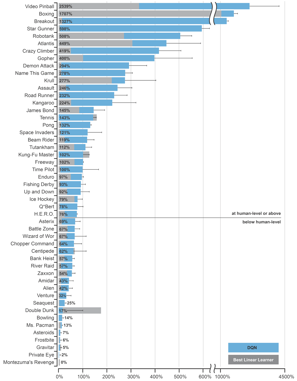
• The DQN network was trained to solve 49 different Atari 2600 games with the same architecture and hyperparameters.

• In most of the games, the network reaches super-human performance.

• Some games are still badly performed (e.g. Montezuma’s revenge), as they require long-term planning.

• It was the first RL algorithm able to learn different tasks (no free lunch theorem).

• The 2015 paper in Nature started the hype for deep RL.

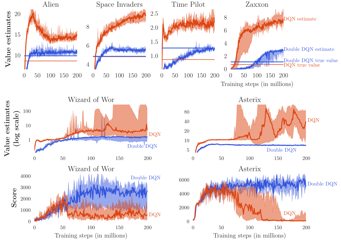
2 - Double DQN

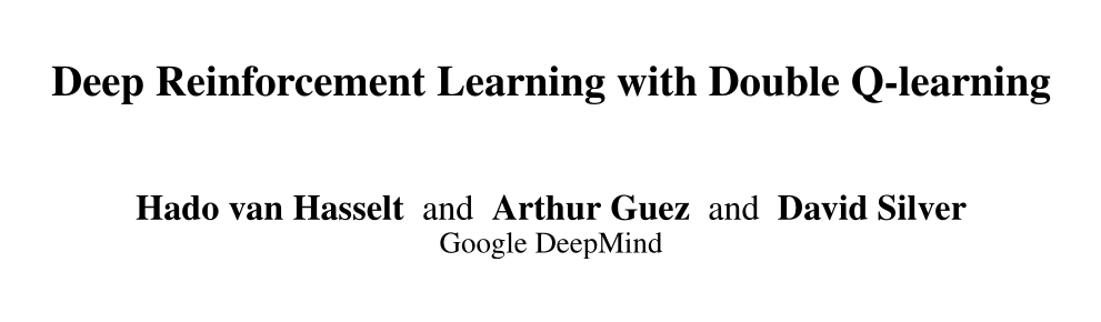
Double DQN

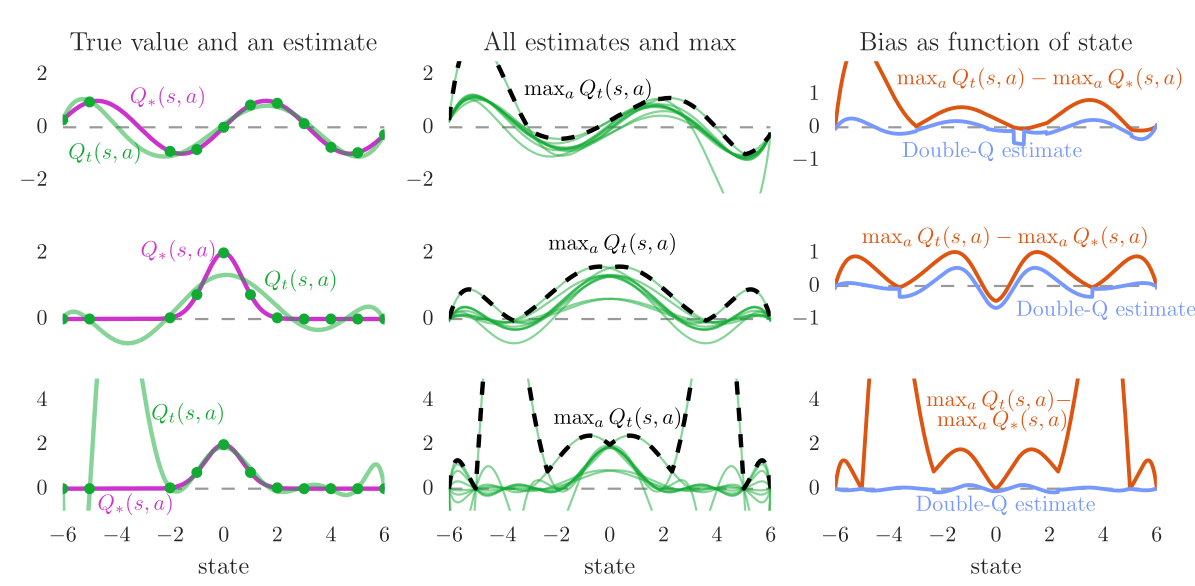
• Q-learning methods, including DQN, tend to overestimate Q-values, especially for the non-greedy actions:

Q_\theta(s, a) > Q^\pi(s, a)

• This does not matter much in action selection, as we apply \epsilon-greedy or softmax on the Q-values anyway, but it may make learning slower (sample complexity) and less optimal.

Double DQN

• To avoid optimistic estimations, the target is computed by both the value network \theta and the target network \theta':

  • Action selection: The next greedy action a^* is calculated by the value network \theta (current policy):

  a^* =\text{argmax}_{a'} Q_{\theta}(s', a')

  • Action evaluation: Its Q-value for the target is calculated using the target network \theta' (older values):

  t = r + \gamma \, Q_{\theta'}(s´, a^*)

• This gives the following loss function for double DQN (DDQN):

\mathcal{L}(\theta) = \mathbb{E}_\mathcal{D} [(r + \gamma \, Q_{\theta'}(s´, \text{argmax}_{a'} Q_{\theta}(s', a')) - Q_\theta(s, a))^2]

3 - Prioritized Experience Replay

Prioritized Experience Replay

Source: https://parksurk.github.io/deep/reinfocement/learning/drlnd_2-4_value_based_methods-post/

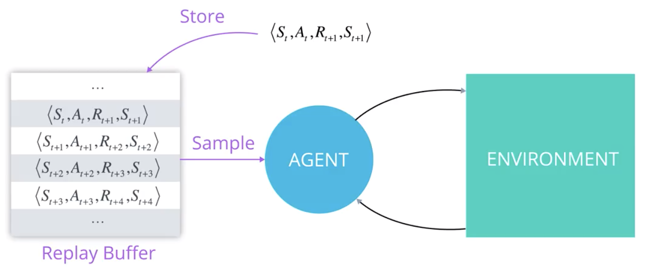
• The experience replay memory or replay buffer is used to store the last 1M transitions (s, a, r, s').

• The learning algorithm randomly samples a minibatch of size K to update its parameters.

• Not all transitions are interesting:

  • Some transitions were generated by a very old policy, the current policy won’t take them anymore.

  • Some transitions are already well predicted: the TD error is small, there is nothing to learn from.

  \delta_t = r_{t+1} + \gamma \, \max_{a'} Q_\theta(s_{t+1}, a_{t+1}) - Q_\theta(s_t, a_t) \approx 0

Prioritized Experience Replay

Source: https://parksurk.github.io/deep/reinfocement/learning/drlnd_2-4_value_based_methods-post/

• The experience replay memory makes learning very slow: we need a lot of samples to learn something useful:

  • High sample complexity.

• We need a smart mechanism to preferentially pick the transitions that will boost learning the most, without introducing a bias.

  • Prioritized sweeping is actually a quite old idea:

Moore and Atkeson (1993). Prioritized sweeping: Reinforcement learning with less data and less time. Machine Learning, 13(1):103–130.

Prioritized Experience Replay

• The idea of prioritized experience replay (PER) is to sample in priority those transitions whose TD error is the highest:

\delta_t = r_{t+1} + \gamma \, \max_{a'} Q_\theta(s_{t+1}, a_{t+1}) - Q_\theta(s_t, a_t)

• In practice, we insert the transition (s, a, r, s', \delta) into the replay buffer.

• To create a minibatch, the sampling algorithm select a transition k based on the probability:

P(k) = \frac{(|\delta_k| + \epsilon)^\alpha}{\sum_k (|\delta_k| + \epsilon)^\alpha}

• \epsilon is a small parameter ensuring that transition with no TD error still get sampled from time to time.

• \alpha allows to change the behavior from uniform sampling (\alpha=0, as in DQN) to fully prioritized sampling (\alpha=1). \alpha should be annealed from 0 to 1 during training.

• Think of it as a “kind of” softmax over the TD errors.

• After the samples have been used for learning, their TD error \delta is updated in the PER.

Prioritized Experience Replay

• The main drawback is that inserting and sampling can be computationally expensive if we simply sort the transitions based on (|\delta_k| + \epsilon)^\alpha:

  • Insertion: \mathcal{O}(N \, \log N).

  • Sampling: \mathcal{O}(N).

Source: https://jaromiru.com/2016/11/07/lets-make-a-dqn-double-learning-and-prioritized-experience-replay/

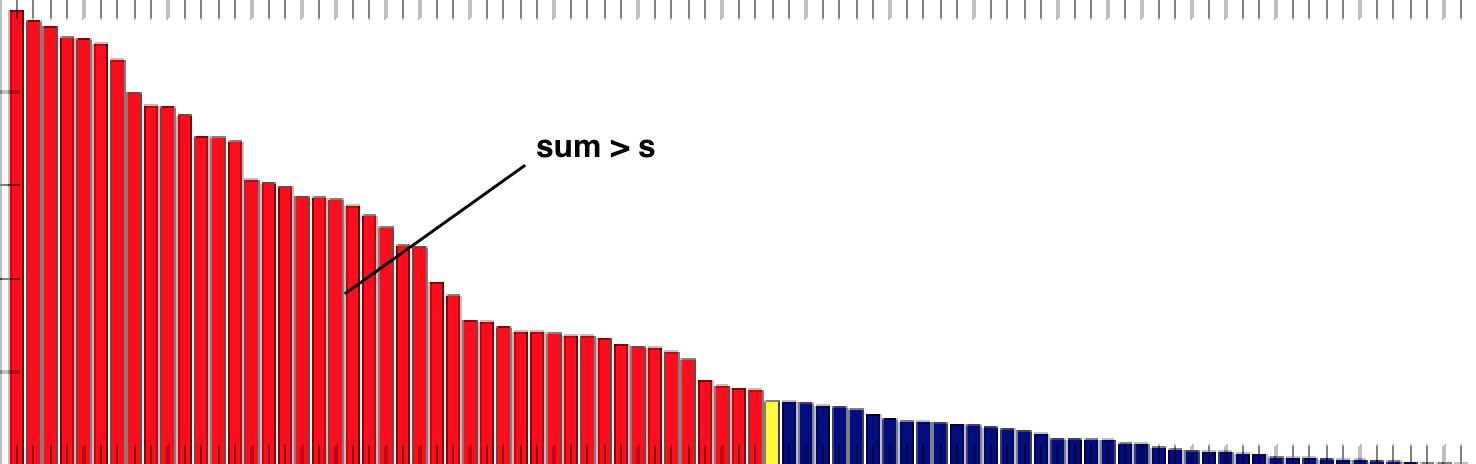
Prioritized Experience Replay

• Using binary sumtrees, prioritized experience replay can be made efficient in both insertion (\mathcal{O}(\log N)) and sampling (\mathcal{O}(1)).

• Instead of a linear queue, we use a binary tree to store the transitions.

• Details in a real computer science course…

Source: https://www.freecodecamp.org/news/improvements-in-deep-q-learning-dueling-double-dqn-prioritized-experience-replay-and-fixed-58b130cc5682/

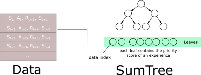
Prioritized Experience Replay

Prioritized Experience Replay

4 - Dueling networks

Dueling networks

• DQN and its variants learn to predict directly the Q-value of each available action.

• Several problems with predicting Q-values with a DNN:

  • The Q-values can take high values, especially with different values of \gamma.

  • The Q-values have a high variance, between the minimum and maximum returns obtained during training.

  • For a transition (s_t, a_t, s_{t+1}), a single Q-value is updated, not all actions in s_t.

Dueling networks

• Enduro game.

Source: https://gfycat.com/clumsypaleimpala

• The exact Q-values of all actions are not equally important.

  • In bad states (low V^\pi(s)), you can do whatever you want, you will lose.

  • In neutral states, you can do whatever you want, nothing happens.

  • In good states (high V^\pi(s)), you need to select the right action to get rewards, otherwise you lose.

Advantage functions

• An important notion is the advantage A^\pi(s, a) of an action:

A^\pi(s, a) = Q^\pi(s, a) - V^\pi(s)

• It tells how much return can be expected by taking the action a in the state s, compared to what is usually obtained in s with the current policy.

• If a policy \pi is deterministic and always selects a^* in s, we have:

A^\pi(s, a^*) = 0 A^\pi(s, a \neq a^*) < 0

• This is particularly true for the optimal policy.

• But if we have separate estimates V_\varphi(s) and Q_\theta(s, a), some actions may have a positive advantage.

• Advantages have less variance than Q-values.

Dueling networks

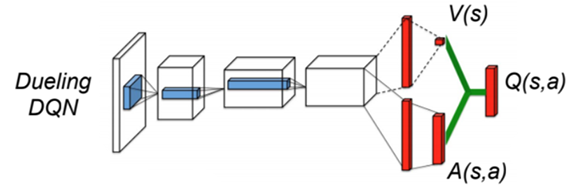
• In dueling networks, the network is forced to decompose the estimated Q-value Q_\theta(s, a) into a state value V_\alpha(s) and an advantage function A_\beta(s, a):

Q_\theta(s, a) = V_\alpha(s) + A_\beta(s, a)

• The parameters \alpha and \beta are just two shared subparts of the NN \theta.

• The loss function

\mathcal{L}(\theta) = \mathbb{E}_\mathcal{D} [(r + \gamma \, Q_{\theta'}(s´, \text{argmax}_{a'} Q_{\theta}(s', a')) - Q_\theta(s, a))^2]

is exactly the same as in (D)DQN: only the internal structure of the NN changes.

Unidentifiability

• The Q-values are the sum of two functions: \; Q_\theta(s, a) = V_\alpha(s) + A_\beta(s, a)

• However, the sum is unidentifiable:

\begin{aligned} Q_\theta(s, a) = 10 & = 1 + 9 \\ & = 2 + 8 \\ & = 3 + 7 \\ \end{aligned}

• To constrain the sum, (Wang et al. 2016) propose that the greedy action w.r.t the advantages should have an advantage of 0:

Q_\theta(s, a) = V_\alpha(s) + (A_\beta(s, a) - \max_{a'} A_\beta(s, a'))

• This way, there is only one solution to the addition. The operation is differentiable, so backpropagation will work.

• (Wang et al. 2016) show that subtracting the mean advantage works better in practice:

Q_\theta(s, a) = V_\alpha(s) + (A_\beta(s, a) - \frac{1}{|\mathcal{A}|} \, \sum_{a'} A_\beta(s, a'))

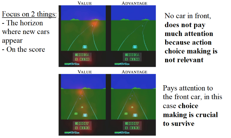
Visualization of the value and advantage functions

• Which pixels change the most the value and advantage functions?

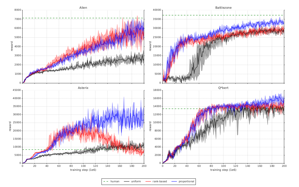
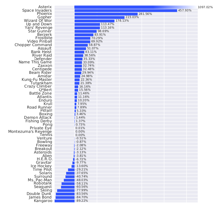
Improvement over prioritized DDQN

Summary of DQN

• DQN and its early variants (double duelling DQN with PER) are an example of value-based deep RL.

• The value Q_\theta(s, a) of each possible action in a given state is approximated by a convolutional neural network.

• The NN has to minimize the mse between the predicted Q-values and the target value corresponding to the Bellman equation:

\mathcal{L}(\theta) = \mathbb{E}_\mathcal{D} [(r + \gamma \, Q_{\theta'}(s´, \text{argmax}_{a'} Q_{\theta}(s', a')) - Q_\theta(s, a))^2]

• The use of an experience replay memory and of target networks allows to stabilize learning and avoid suboptimal policies.

• The main drawback of DQN is sample complexity: it needs huge amounts of experienced transitions to find a correct policy. The sample complexity come from the deep network itself (gradient descent is iterative and slow), but also from the ERM: it contains 1M transitions, most of which are outdated.

• Only works for small and discrete action spaces (one output neuron per action).