Deep Reinforcement Learning
Deep Deterministic Policy Gradient
1 - Deterministic policy gradient theorem
Deterministic policy gradient theorem
- The objective function that we tried to maximize until now is :
\mathcal{J}(\theta) = \mathbb{E}_{\tau \sim \rho_\theta}[R(\tau)]
i.e. we want the returns of all trajectories generated by the stochastic policy \pi_\theta to be maximal.
- It is equivalent to say that we want the value of all states visited by the policy \pi_\theta to be maximal:
a policy \pi is better than another policy \pi' if its expected return is greater or equal than that of \pi' for all states s.
\pi > \pi' \Leftrightarrow V^{\pi}(s) > V^{\pi'}(s) \quad \forall s \in \mathcal{S}

- The objective function can be rewritten as:
\mathcal{J}'(\theta) = \mathbb{E}_{s \sim \rho_\theta}[V^{\pi_\theta}(s)]
where \rho_\theta is now the state visitation distribution, i.e. how often a state will be visited by the policy \pi_\theta.
Deterministic policy gradient theorem
- The policy gradient for the deterministic policy \mu_\theta(s) becomes:
g = \nabla_\theta \, \mathcal{J}(\theta) = \mathbb{E}_{s \sim \rho_\theta}[\nabla_\theta \, Q^{\mu_\theta}(s, \mu_\theta(s))]
- We can now use the chain rule to decompose the gradient of Q^{\mu_\theta}(s, \mu_\theta(s)):
\nabla_\theta \, Q^{\mu_\theta}(s, \mu_\theta(s)) = \nabla_a \, Q^{\mu_\theta}(s, a)|_{a = \mu_\theta(s)} \times \nabla_\theta \, \mu_\theta(s)
\nabla_a \, Q^{\mu_\theta}(s, a)|_{a = \mu_\theta(s)} means that we differentiate Q^{\mu_\theta} w.r.t. a, and evaluate it in \mu_\theta(s).
- a is a variable, but \mu_\theta(s) is a deterministic value (constant).
\nabla_\theta \, \mu_\theta(s) tells how the output of the policy network varies with the parameters of NN:
- Automatic differentiation frameworks such as tensorflow can tell you that.
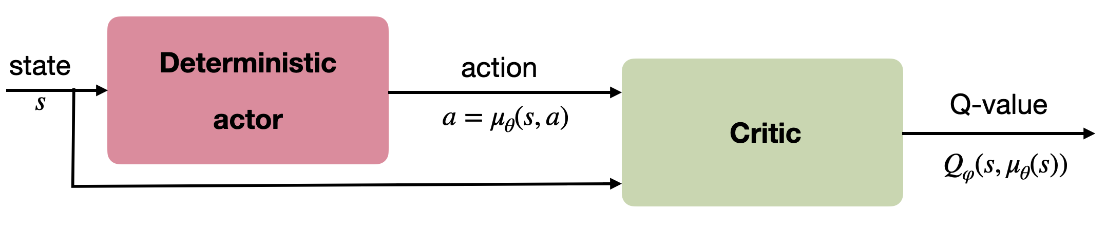
Deterministic Policy Gradient as an actor-critic architecture
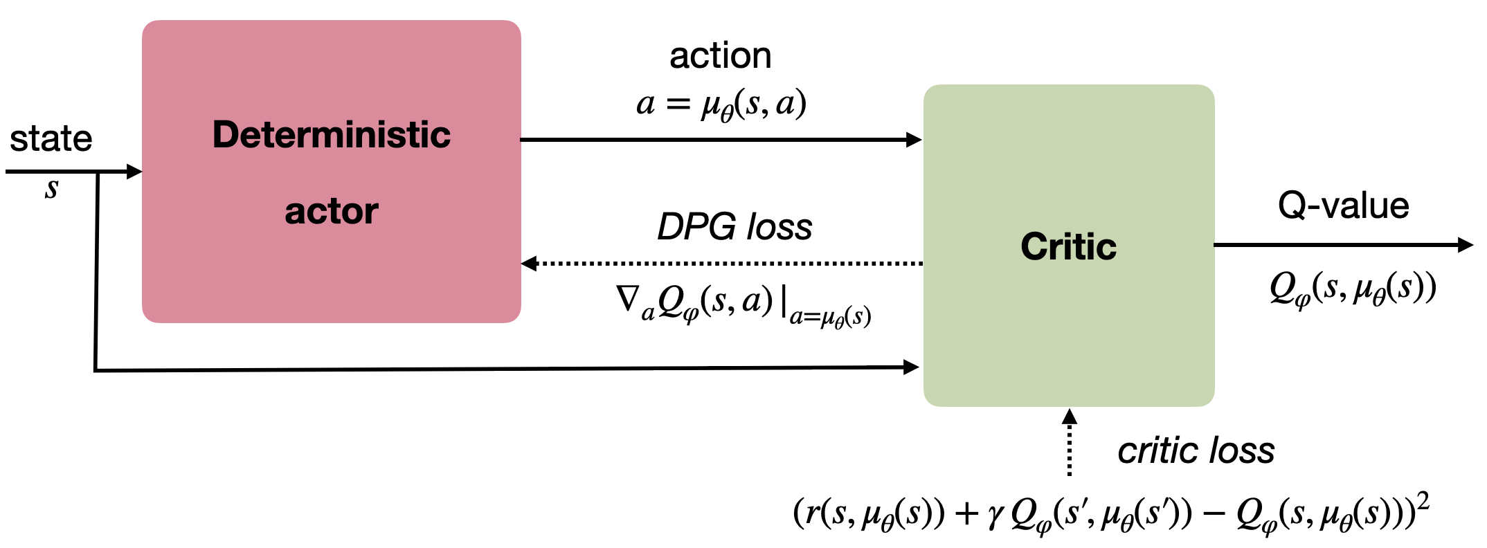
Training the actor:
\nabla_\theta \mathcal{J}(\theta) = \mathbb{E}_{s \sim \rho_\theta}[\nabla_\theta \, \mu_\theta(s) \times \nabla_a Q_\varphi(s, a) |_{a = \mu_\theta(s)}]
Training the critic:
\mathcal{L}(\varphi) = \mathbb{E}_{s \sim \rho_\theta}[(r(s, \mu_\theta(s)) + \gamma \, Q_\varphi(s', \mu_\theta(s')) - Q_\varphi(s, \mu_\theta(s)))^2]
2 - DDPG: Deep Deterministic Policy Gradient
DDPG: Deep Deterministic Policy Gradient
As the name indicates, DDPG is the deep variant of DPG for continuous control.
It uses the DQN tricks to stabilize learning with deep networks:
As DPG is off-policy, an experience replay memory can be used to sample experiences.
The actor \mu_\theta learns using sampled transitions with DPG.
The critic Q_\varphi uses Q-learning on sampled transitions: target networks can be used to cope with the non-stationarity of the Bellman targets.
- Contrary to DQN, the target networks are not updated every once in a while, but slowly integrate the trained networks after each update (moving average of the weights):
\theta' \leftarrow \tau \theta + (1-\tau) \, \theta'
\varphi' \leftarrow \tau \varphi + (1-\tau) \, \varphi'
DDPG: Deep Deterministic Policy Gradient
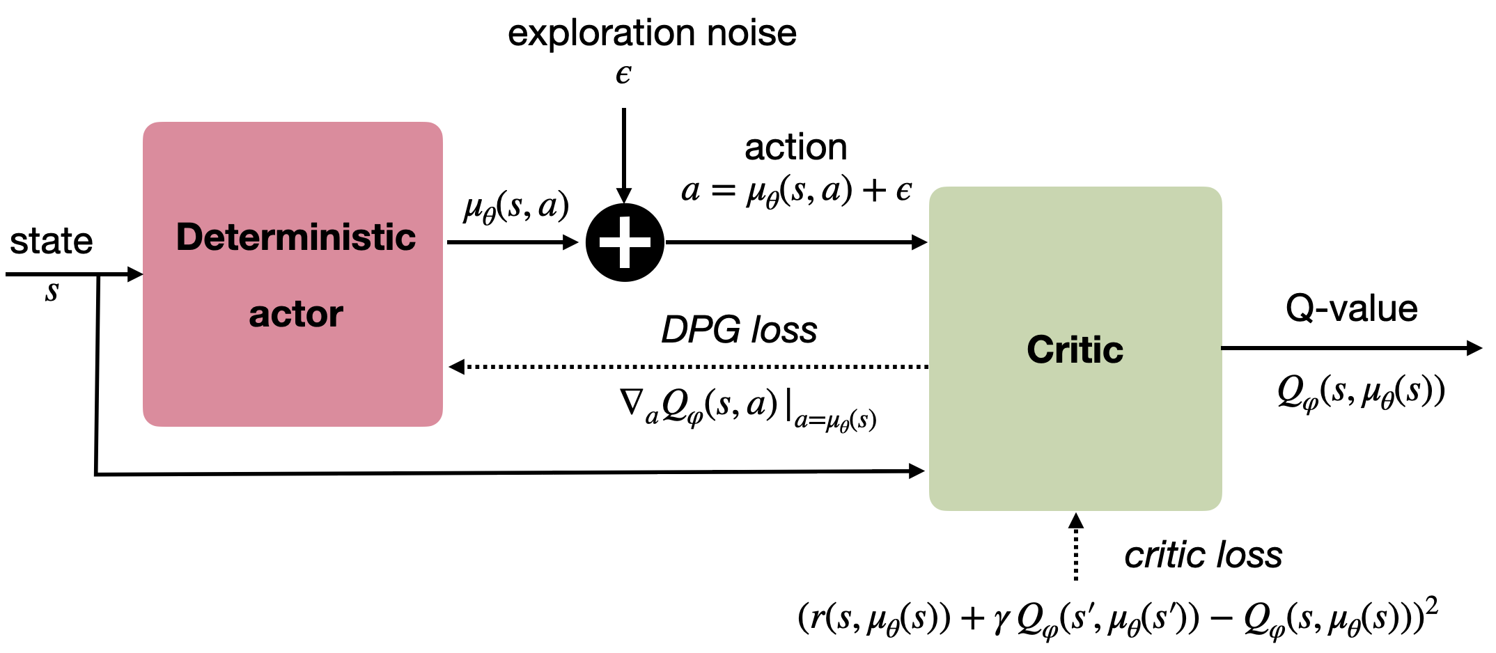
A deterministic actor is good for learning (less variance), but not for exploring.
We cannot use \epsilon-greedy or softmax, as the actor outputs directly the policy, not Q-values.
For continuous actions, an exploratory noise can be added to the deterministic action:
a_t = \mu_\theta(s_t) + \xi_t
- Ex: if the actor wants to move the joint of a robot by 2^o, it will actually be moved from 2.1^o or 1.9^o.
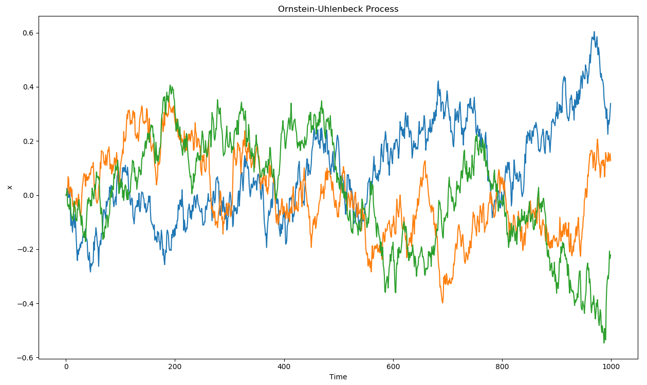
Ornstein-Uhlenbeck stochastic process
In DDPG, an Ornstein-Uhlenbeck stochastic process is used to add noise to the continuous actions.
It is defined by a stochastic differential equation, classically used to describe Brownian motion:
dx_t = \theta (\mu - x_t) dt + \sigma dW_t \qquad \text{with} \qquad dW_t = \mathcal{N}(0, dt)
- The temporal mean of x_t is \mu= 0, its amplitude is \theta (exploration level), its speed is \sigma.
Parameter noise
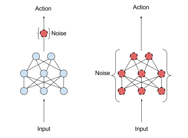
Another approach to ensure exploration is to add noise to the parameters \theta of the actor at inference time.
For the same input s_t, the output \mu_\theta(s_t) will be different every time.
The NoisyNet approach can be applied to any deep RL algorithm to enable a smart state-dependent exploration (e.g. Noisy DQN).
DDPG: Deep Deterministic Policy Gradient
DDPG allows to learn continuous policies: there can be one tanh output neuron per joint in a robot.
The learned policy is deterministic: this simplifies learning as we do not need to integrate over the action space after sampling.
Exploratory noise (e.g. Ohrstein-Uhlenbeck) has to be added to the selected action during learning in order to ensure exploration.
Allows to use an experience replay memory, reusing past samples (better sample complexity than A3C).
3 - DDPG: learning to drive in a day
DDPG: learning to drive in a day
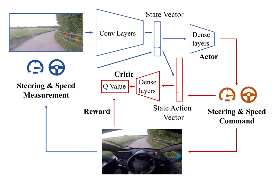
The algorithm is DDPG with prioritized experience replay.
Training is live, with an on-board NVIDIA Drive PX2 GPU.
A simulated environment is first used to find the hyperparameters.
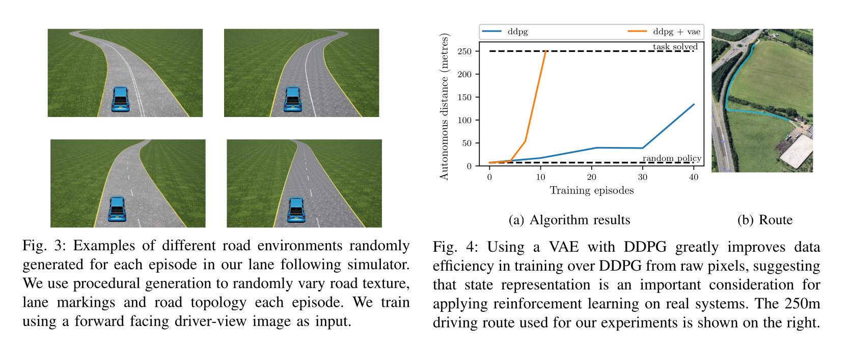
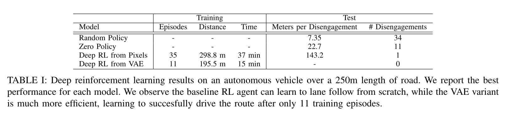
Autoencoders in deep RL
- A variational autoencoder (VAE) is optionally use to pretrain the convolutional layers on random episodes.

DDPG: learning to drive in a day
4 - TD3 - Twin Delayed Deep Deterministic policy gradient
TD3 - Twin Delayed Deep Deterministic policy gradient
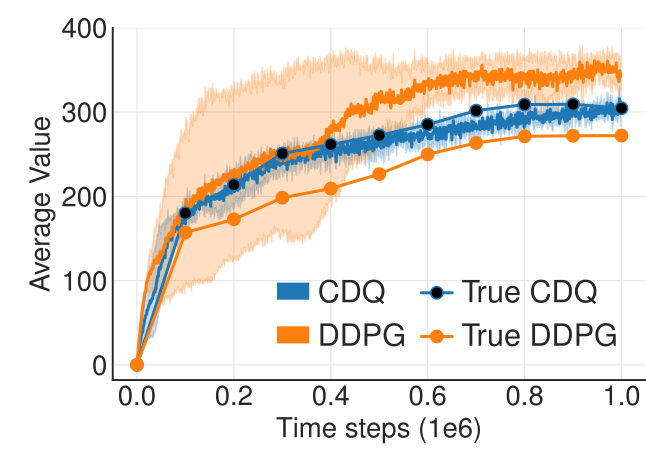
As any Q-learning-based method, DDPG overestimates Q-values.
The Bellman target t = r + \gamma \, \max_{a'} Q(s', a') uses a maximum over other values, so it is increasingly overestimated during learning.
After a while, the overestimated Q-values disrupt training in the actor.
- Double Q-learning solves the problem by using the target network \theta' to estimate Q-values, but the value network \theta to select the greedy action in the next state:
\mathcal{L}(\theta) = \mathbb{E}_\mathcal{D} [(r + \gamma \, Q_{\theta'}(s´, \text{argmax}_{a'} Q_{\theta}(s', a')) - Q_\theta(s, a))^2]
The idea is to use two different independent networks to reduce overestimation.
This does not work well with DDPG, as the Bellman target t = r + \gamma \, Q_{\varphi'}(s', \mu_{\theta'}(s')) uses a target actor network that is not very different from the trained deterministic actor.
TD3 - Twin Delayed Deep Deterministic policy gradient
- Another issue with actor-critic architecture in general is that the critic is always biased during training, what can impact the actor and ultimately collapse the policy:
\nabla_\theta \mathcal{J}(\theta) = \mathbb{E}[ \nabla_\theta \mu_\theta(s) \times \nabla_a Q_{\varphi_1}(s, a) |_{a = \mu_\theta(s)} ]
Q_{\varphi_1}(s, a) \approx Q^{\mu_\theta}(s, a)
- The critic should learn much faster than the actor in order to provide unbiased gradients.

Increasing the learning rate in the critic creates instability, reducing the learning rate in the actor slows down learning.
The solution proposed by TD3 is to delay the update of the actor, i.e. update it only every d minibatches:
Train the critics \varphi_1 and \varphi_2 on the minibatch.
every d steps:
- Train the actor \theta on the minibatch.
This leaves enough time to the critics to improve their prediction and provides less biased gradients to the actor.
TD3 - Twin Delayed Deep Deterministic policy gradient
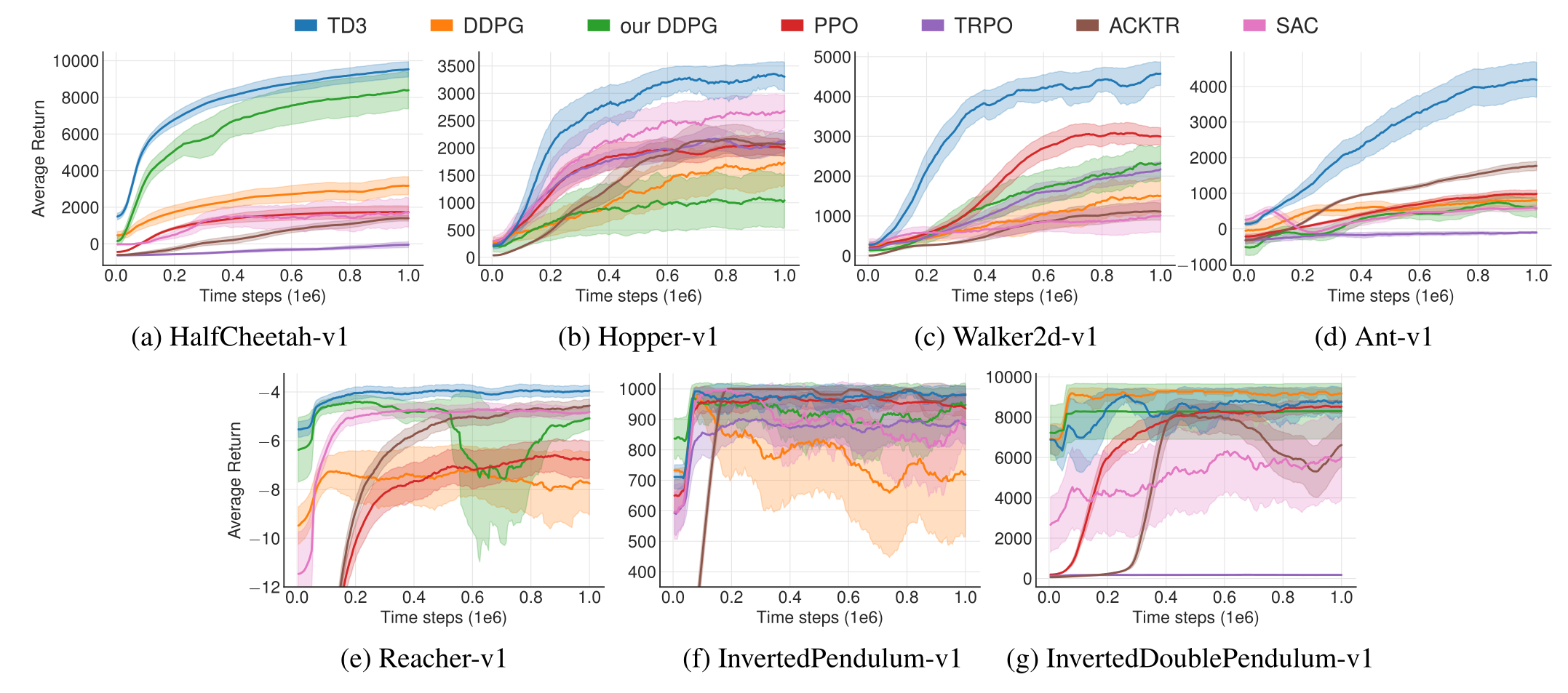
TD3 introduces three changes to DDPG:
- twin critics.
- delayed actor updates.
- noisy Bellman targets.
- TD3 outperforms DDPG (but also PPO and SAC) on continuous control tasks.
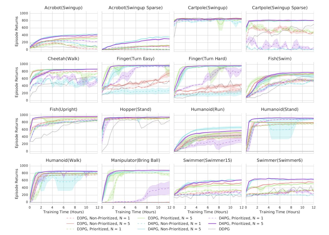
5 - D4PG: Distributed Distributional DDPG
Parkour networks
For Parkour tasks, the states cover two different informations: the terrain (distance to obstacles, etc.) and the proprioception (joint positions of the agent).
They enter the actor and critic networks at different locations.
