Deep Reinforcement Learning
A3C - DDPG - PPO
1 - A3C: Asynchronous advantage actor-critic
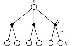
Advantage actor-critic

Advantage actor-critic
The advantage actor-critic is strictly on-policy:
The critic must evaluate actions selected the current version of the actor \pi_\theta, not an old version or another policy.
The actor must learn from the current value function V^{\pi_\theta} \approx V_\varphi.
\begin{cases} \nabla_\theta \mathcal{J}(\theta) = \mathbb{E}_{s_t \sim \rho_\theta, a_t \sim \pi_\theta}[\nabla_\theta \log \pi_\theta (s_t, a_t) \, (R^n_t - V_\varphi(s_t)) ] \\ \\ \mathcal{L}(\varphi) = \mathbb{E}_{s_t \sim \rho_\theta, a_t \sim \pi_\theta}[(R^n_t - V_\varphi(s_t))^2] \\ \end{cases}
- We cannot use an experience replay memory to deal with the correlated inputs, as it is only for off-policy methods.
Distributed RL
- We cannot get an uncorrelated batch of transitions by acting sequentially with a single agent.

- A simple solution is to have multiple actors with the same weights \theta interacting in parallel with different copies of the environment. See GORILA, APE-X, R2D2.

Each rollout worker (actor) starts an episode in a different state: at any point of time, the workers will be in uncorrelated states.
From time to time, the workers all send their experienced transitions to the learner which updates the policy using a batch of uncorrelated transitions.
After the learner update, the workers use the new policy to collect new transitions.
A3C: Asynchronous advantage actor-critic
- In A3C, the workers do not simply collect experiences, but also compute gradients on their collected transitions and send them to the global network.
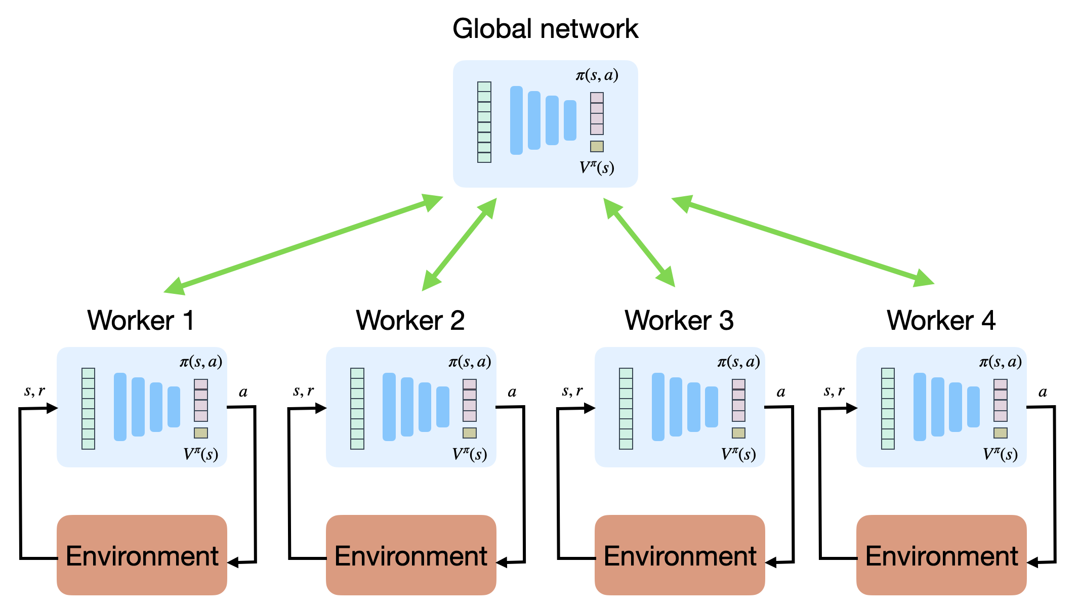
A3C: Asynchronous advantage actor-critic
A3C does not use an experience replay memory as DQN.
Instead, it uses multiple parallel workers to distribute learning.
Each worker has a copy of the actor and critic networks, as well as an instance of the environment.
Weight updates are synchronized regularly though a master network using Hogwild!-style updates (every n=5 steps!).
Because the workers learn different parts of the state-action space, the weight updates are not very correlated.
- It works best on shared-memory systems (multi-core) as communication costs between GPUs are huge.
A3C : results
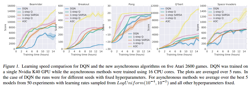
A3C set a new record for Atari games in 2016.
The main advantage is that the workers gather experience in parallel: training is much faster than with DQN.
LSTMs can be used to improve the performance.
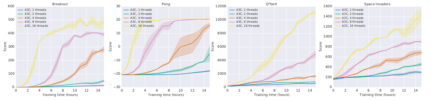
A3C : results
- Learning is only marginally better with more threads:
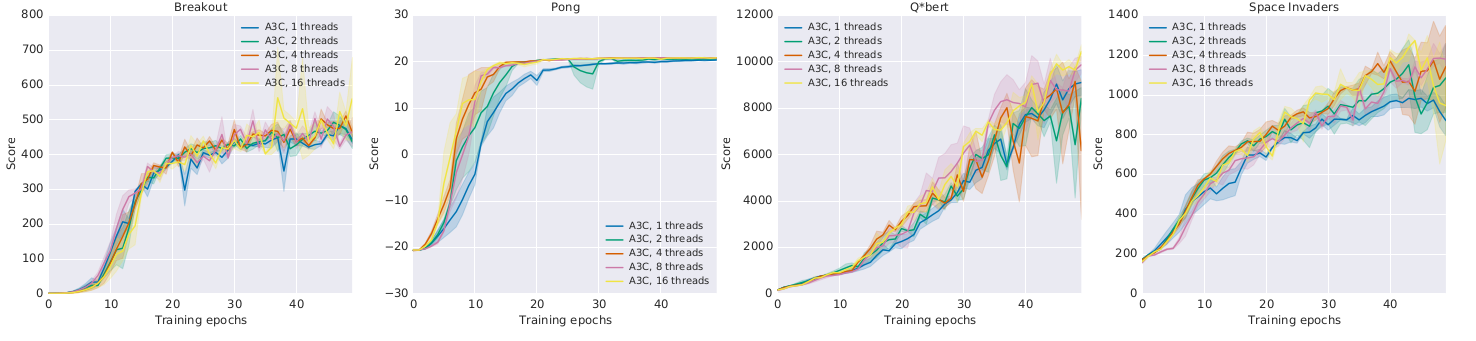
but much faster!
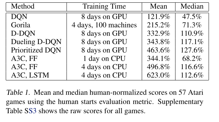
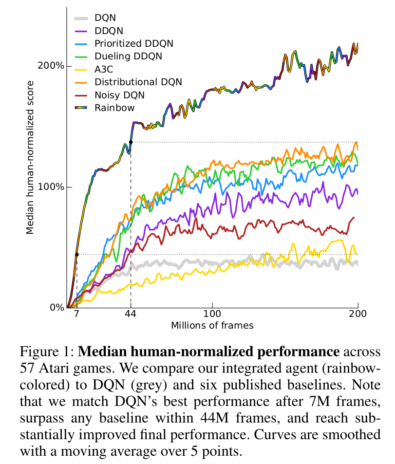
Comparison with DQN
- A3C came up in 2016. A lot of things happened since then…
2 - DDPG: Deep Deterministic Policy Gradient
Deterministic policy gradient theorem
- The objective function that we tried to maximize until now is :
\mathcal{J}(\theta) = \mathbb{E}_{\tau \sim \rho_\theta}[R(\tau)]
i.e. we want the returns of all trajectories generated by the stochastic policy \pi_\theta to be maximal.
It is equivalent to say that we want the value of all states visited by the policy \pi_\theta to be maximal:
- a policy \pi is better than another policy \pi' if its expected return is greater or equal than that of \pi' for all states s.
\pi > \pi' \Leftrightarrow V^{\pi}(s) > V^{\pi'}(s) \quad \forall s \in \mathcal{S}

- The objective function can be rewritten as:
\mathcal{J}'(\theta) = \mathbb{E}_{s \sim \rho_\theta}[V^{\pi_\theta}(s)]
where \rho_\theta is now the state visitation distribution, i.e. how often a state will be visited by the policy \pi_\theta.
Deterministic policy gradient theorem
- When introducing Q-values in each state, we obtain the following policy gradient:
g = \nabla_\theta \, \mathcal{J}(\theta) = \mathbb{E}_{s \sim \rho_\theta}[\nabla_\theta \, V^{\pi_\theta}(s)] = \mathbb{E}_{s \sim \rho_\theta}[\nabla_\theta \, \sum_a \pi_\theta(s, a) \, Q^{\pi_\theta}(s, a)]
This formulation necessitates to integrate overall possible actions:
Not possible with continuous action spaces.
The stochastic policy adds a lot of variance.
What would happen if the policy were deterministic, i.e. it always takes a single action in state s?
We can note this deterministic policy \mu_\theta(s), with:
\begin{aligned} \mu_\theta : \; \mathcal{S} & \rightarrow \mathcal{A} \\ s & \; \rightarrow \mu_\theta(s) \\ \end{aligned}
- The policy gradient becomes only stochastic regarding the visited states:
g = \nabla_\theta \, \mathcal{J}(\theta) = \mathbb{E}_{s \sim \rho_\theta}[\nabla_\theta \, Q^{\mu_\theta}(s, \mu_\theta(s))]
Deterministic policy gradient theorem

- The deterministic policy gradient is:
g = \nabla_\theta \, \mathcal{J}(\theta) = \mathbb{E}_{s \sim \rho_\theta}[\nabla_\theta \, Q^{\pi_\theta}(s, \mu_\theta(s))]
- We can now use the chain rule to decompose the gradient of Q^{\mu_\theta}(s, \mu_\theta(s)):
\nabla_\theta \, Q^{\mu_\theta}(s, \mu_\theta(s)) = \nabla_a \, Q^{\mu_\theta}(s, a)|_{a = \mu_\theta(s)} \times \nabla_\theta \, \mu_\theta(s)
\nabla_a \, Q^{\mu_\theta}(s, a)|_{a = \mu_\theta(s)} means that we differentiate Q^{\mu_\theta} w.r.t. a, and evaluate it in \mu_\theta(s).
- a is a variable, but \mu_\theta(s) is a deterministic value (constant).
\nabla_\theta \, \mu_\theta(s) tells how the output of the policy network varies with the parameters of NN:
- Automatic differentiation frameworks such as tensorflow can tell you that.
Deterministic Policy Gradient as an actor-critic architecture

Training the actor:
\nabla_\theta \mathcal{J}(\theta) = \mathbb{E}_{s \sim \rho_\theta}[\nabla_\theta \, \mu_\theta(s) \times \nabla_a Q_\varphi(s, a) |_{a = \mu_\theta(s)}]
Training the critic:
\mathcal{L}(\varphi) = \mathbb{E}_{s \sim \rho_\theta}[(r(s, \mu_\theta(s)) + \gamma \, Q_\varphi(s', \mu_\theta(s')) - Q_\varphi(s, \mu_\theta(s)))^2]
DDPG: Deep Deterministic Policy Gradient
As DDPG is off-policy, an experience replay memory can be used to sample experiences.
The actor \mu_\theta learns using sampled transitions with DPG.
The critic Q_\varphi uses Q-learning on sampled transitions: target networks can be used to cope with the non-stationarity of the Bellman targets.
- Contrary to DQN, the target networks are not updated every once in a while, but slowly integrate the trained networks after each update (moving average of the weights):
\theta' \leftarrow \tau \theta + (1-\tau) \, \theta'
\varphi' \leftarrow \tau \varphi + (1-\tau) \, \varphi'
DDPG: Deep Deterministic Policy Gradient

A deterministic actor is good for learning (less variance), but not for exploring.
We cannot use \epsilon-greedy or softmax, as the actor outputs directly the policy, not Q-values.
For continuous actions, an exploratory noise can be added to the deterministic action:
a_t = \mu_\theta(s_t) + \xi_t
Ex: if the actor wants to move the joint of a robot by 2^o, it will actually be moved from 2.1^o or 1.9^o.
Ornstein-Uhlenbeck stochastic processes or parameter noise can be used for exploration.
DDPG: learning to drive in a day
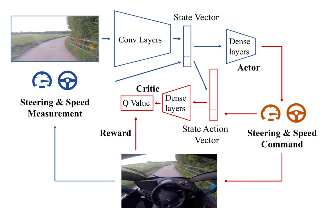
The algorithm is DDPG with prioritized experience replay. The Convnet is pretrained using an autoencoder.
Training is live, with an on-board NVIDIA Drive PX2 GPU.
A simulated environment is first used to find the hyperparameters.
3 - PPO: Proximal Policy Optimization
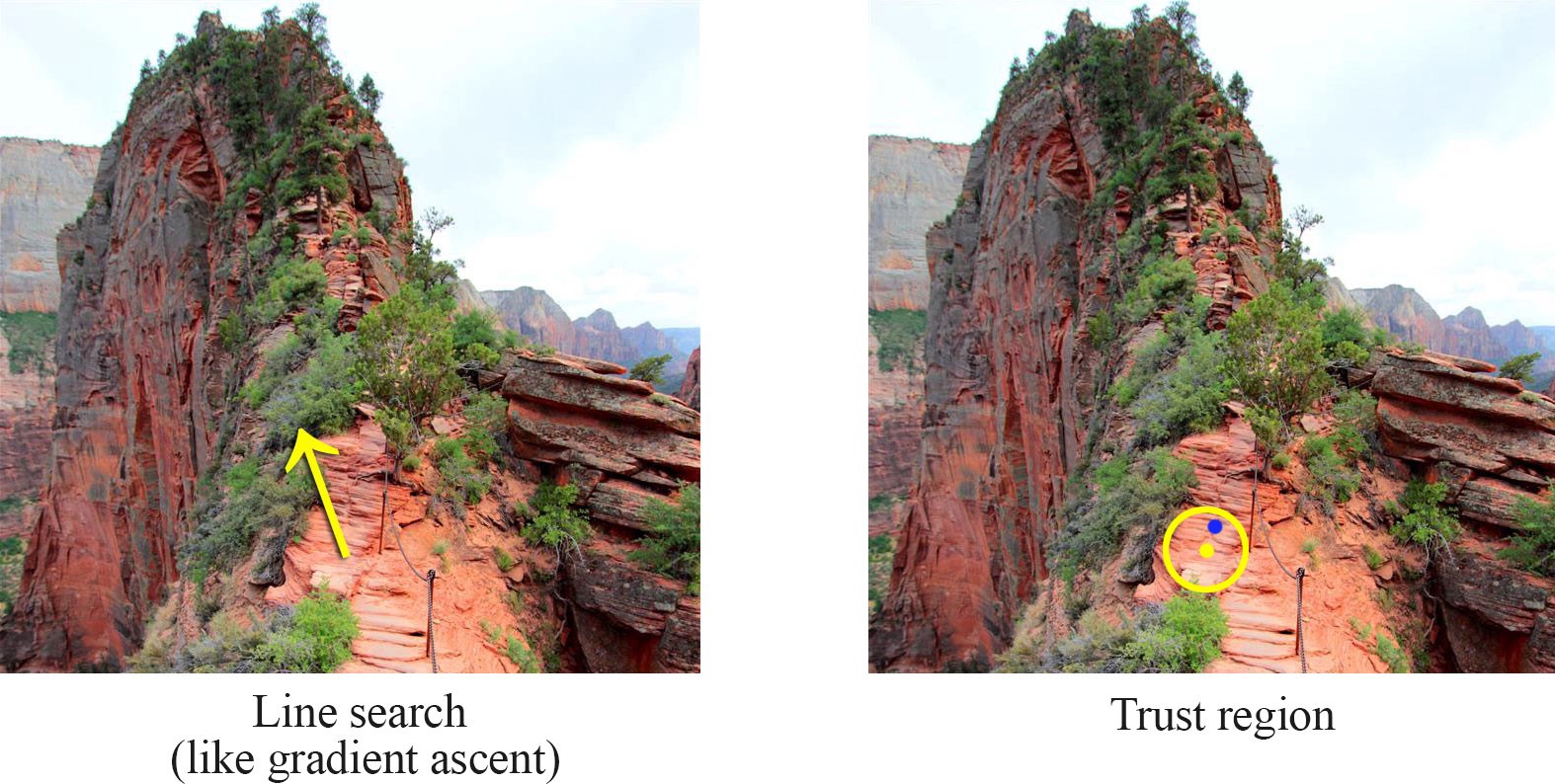
Trust regions and gradients
Source: https://medium.com/@jonathan_hui/rl-trust-region-policy-optimization-trpo-explained-a6ee04eeeee9
The policy gradient tells you in which direction of the parameter space \theta the return is increasing the most.
If you take too big a step in that direction, the new policy might become completely bad (policy collapse).
Once the policy has collapsed, the new samples will all have a small return: the previous progress is lost.
This is especially true when the parameter space has a high curvature, which is the case with deep NN.
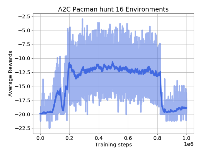
Policy collapse
Policy collapse is a huge problem in deep RL: the network starts learning correctly but suddenly collapses to a random agent.
For on-policy methods, all progress is lost: the network has to relearn from scratch, as the new samples will be generated by a bad policy.
Trust regions and gradients
Reducing the learning rate only leads to slower learning (sample complexity), not safer convergence.
Trust region optimization searches in the neighborhood of the current parameters \theta which new value would maximize the return the most.
This is a constrained optimization problem: we still want to maximize the return of the policy, but by keeping the policy as close as possible from its previous value.
Source: https://medium.com/@jonathan_hui/rl-trust-region-policy-optimization-trpo-explained-a6ee04eeeee9
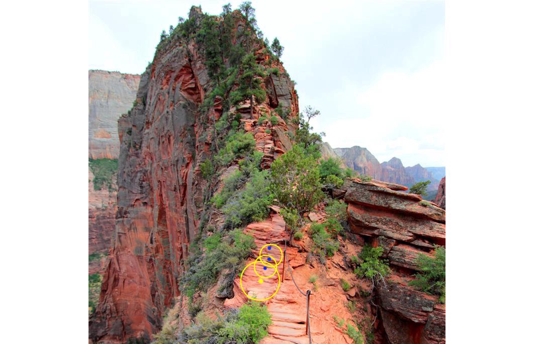
Trust regions and gradients
The size of the neighborhood determines the safety of the parameter change.
In safe regions, we can take big steps. In dangerous regions, we have to take small steps.
Problem: how can we estimate the safety of a parameter change?
Source: https://medium.com/@jonathan_hui/rl-trust-region-policy-optimization-trpo-explained-a6ee04eeeee9
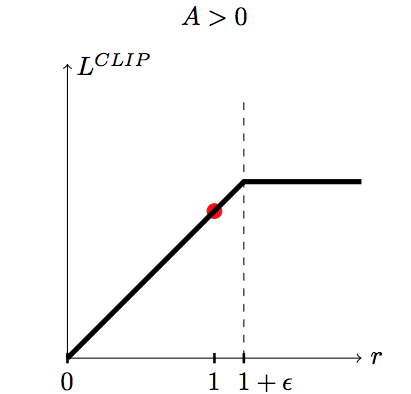
PPO: Proximal Policy Optimization
- The solution introduced by PPO is simply to clip the importance sampling weight when it is too different from 1:
\mathcal{L}(\theta) = \mathbb{E}_{s \sim \rho_{\theta_\text{old}}, a \sim \pi_{\theta_\text{old}}} [\min(\rho(s, a) \, A^{\pi_{\theta_\text{old}}}(s, a), \text{clip}(\rho(s, a), 1-\epsilon, 1+\epsilon) \, A^{\pi_{\theta_\text{old}}}(s, a))]
For each sampled action (s, a), we use the minimum between:
the unconstrained objective with IS \rho(s, a) \, A^{\pi_{\theta_\text{old}}}(s, a).
the same, but with the IS weight clipped between 1-\epsilon and 1+\epsilon.

PPO: Proximal Policy Optimization
If the advantage A^{\pi_{\theta_\text{old}}}(s, a) is positive (better action than usual) and:
the IS is higher than 1+\epsilon, we use
(1+\epsilon) \, A^{\pi_{\theta_\text{old}}}(s, a).otherwise, we use \rho(s, a) \, A^{\pi_{\theta_\text{old}}}(s, a).
If the advantage A^{\pi_{\theta_\text{old}}}(s, a) is negative (worse action than usual) and:
the IS is lower than 1-\epsilon, we use
(1-\epsilon) \, A^{\pi_{\theta_\text{old}}}(s, a).otherwise, we use \rho(s, a) \, A^{\pi_{\theta_\text{old}}}(s, a).
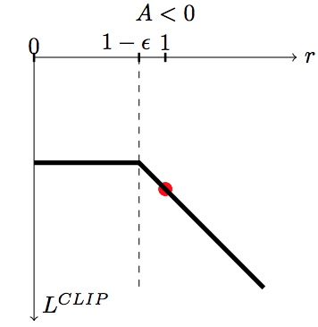
This avoids changing too much the policy between two updates:
Good actions (A^{\pi_{\theta_\text{old}}}(s, a) > 0) do not become much more likely than before.
Bad actions (A^{\pi_{\theta_\text{old}}}(s, a) < 0) do not become much less likely than before.
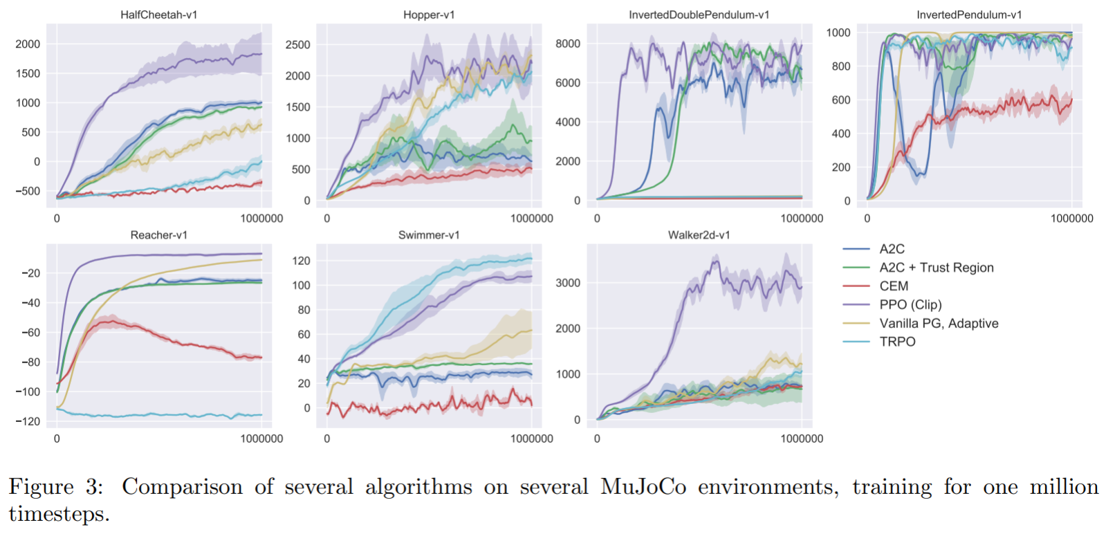
PPO : Mujoco control
PPO: ChatGPT

Why is Dota 2 hard?
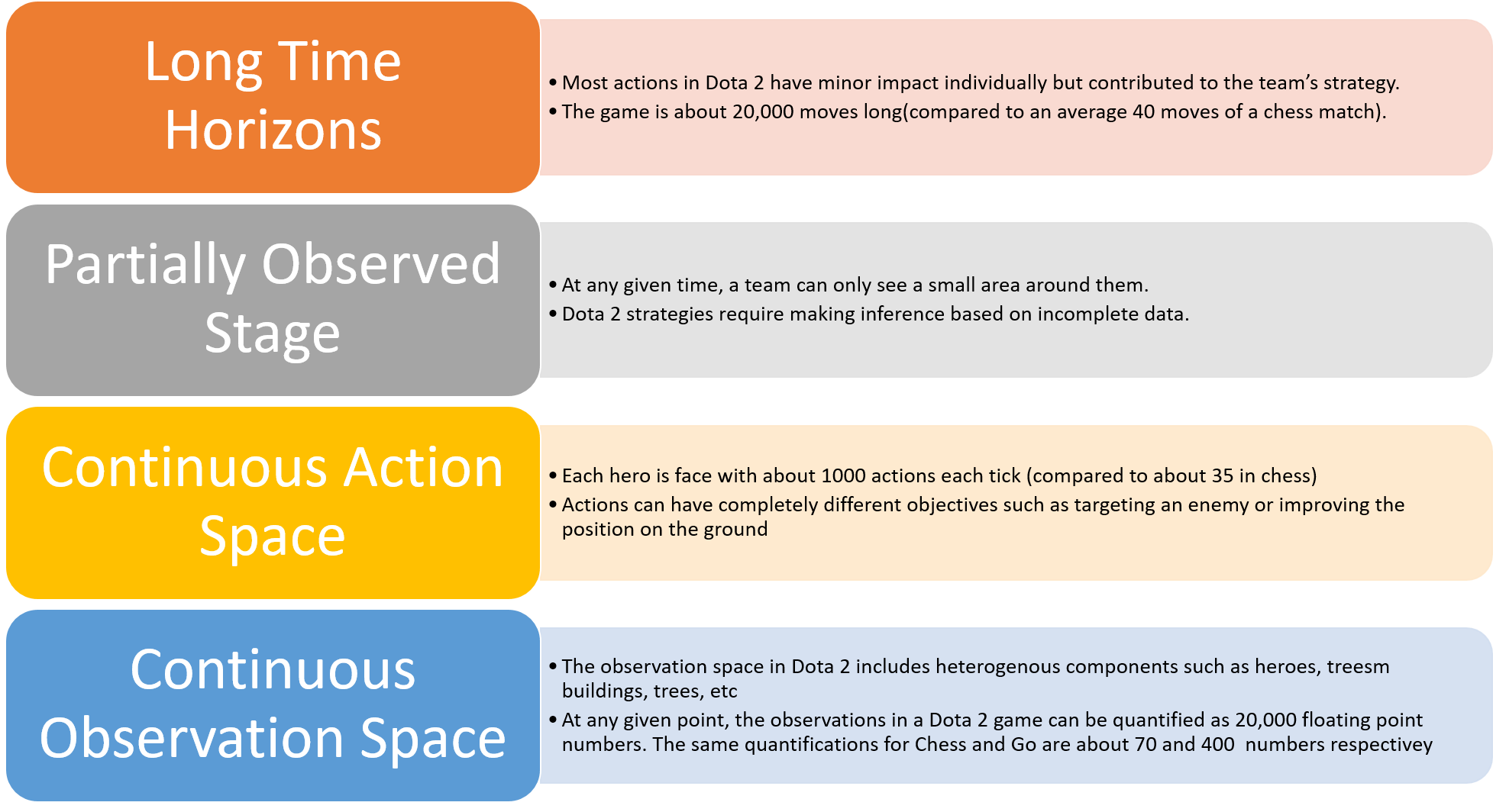
| Feature | Chess | Go | Dota 2 |
|---|---|---|---|
| Total number of moves | 40 | 150 | 20000 |
| Number of possible actions | 35 | 250 | 1000 |
| Number of inputs | 70 | 400 | 20000 |
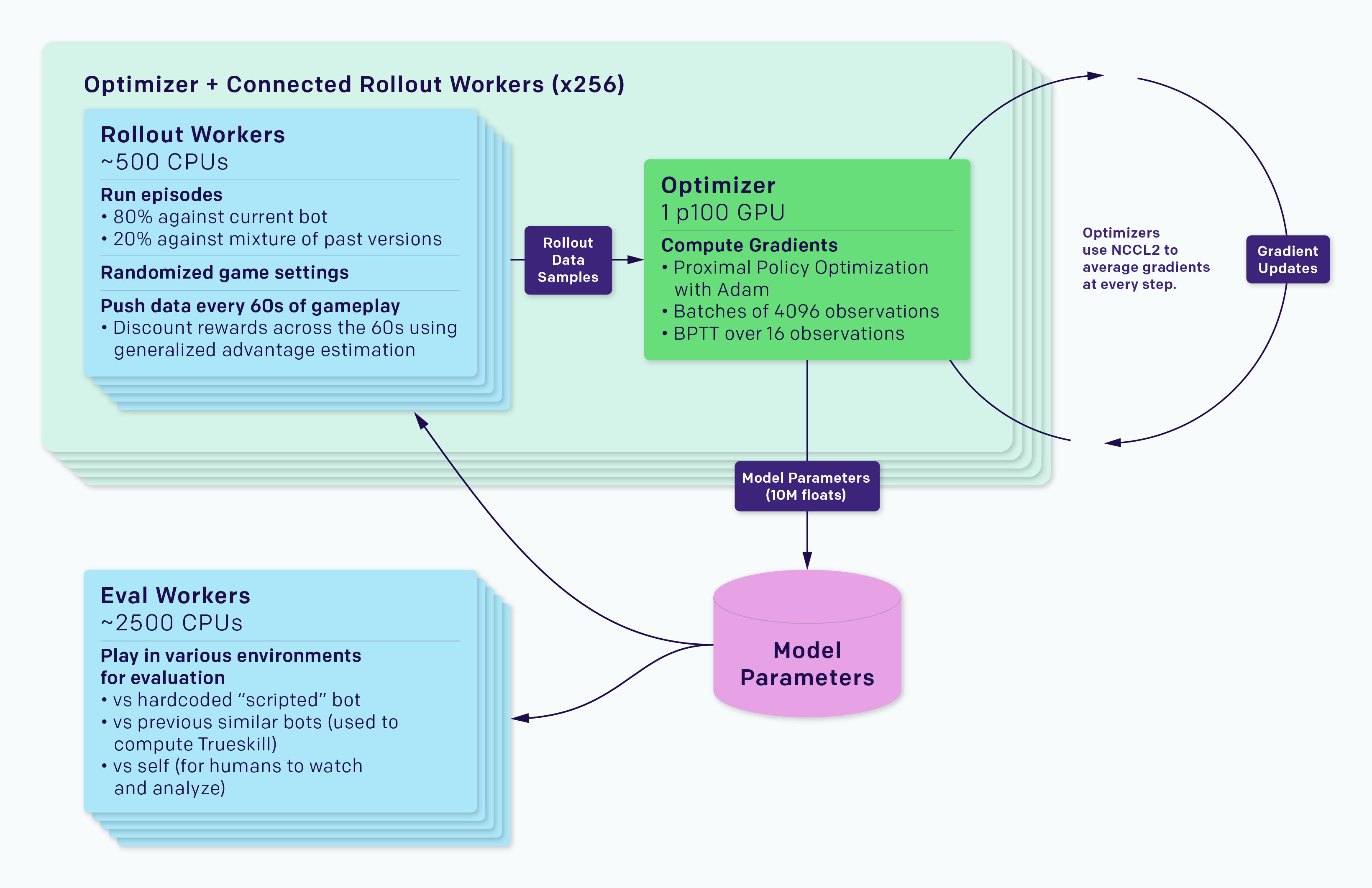
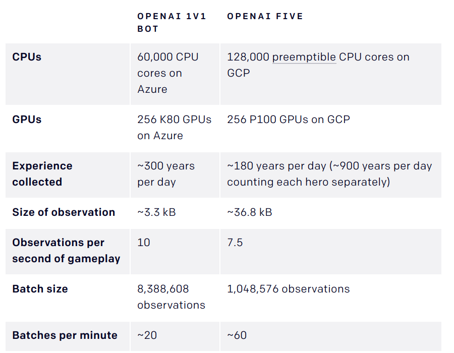
OpenAI Five: Dota 2
- OpenAI Five is composed of 5 PPO networks (one per player), using 128,000 CPUs and 256 V100 GPUs.
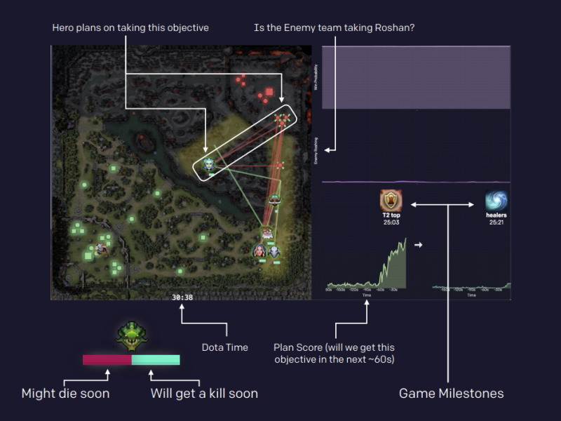
OpenAI Five: Dota 2
OpenAI Five: Dota 2
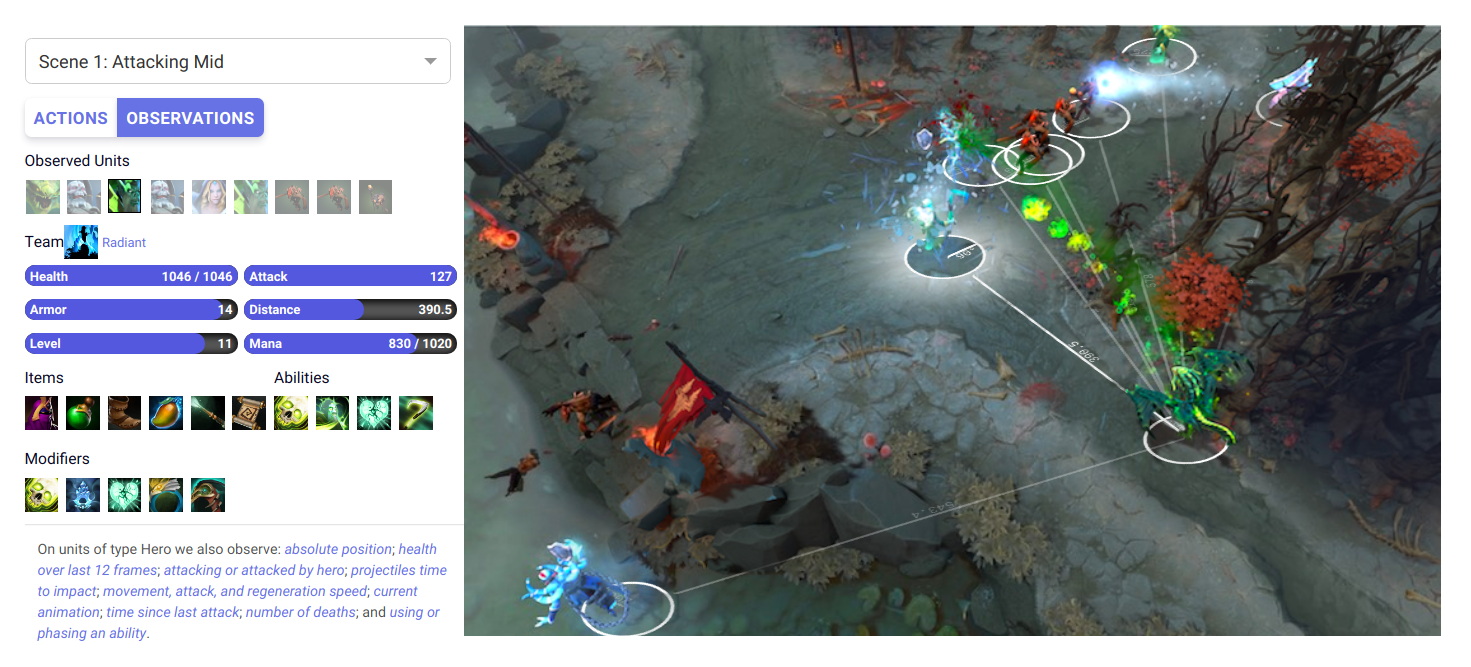
OpenAI Five: Dota 2
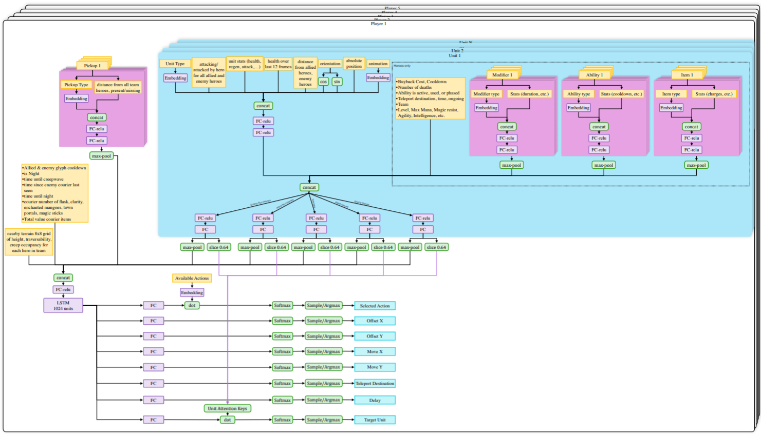
https://d4mucfpksywv.cloudfront.net/research-covers/openai-five/network-architecture.pdf
OpenAI Five: Dota 2
The agents are trained by self-play. Each worker plays against:
the current version of the network 80% of the time.
an older version of the network 20% of the time.
Reward is hand-designed using human heuristics:
- net worth, kills, deaths, assists, last hits…
The discount factor \gamma is annealed from 0.998 (valuing future rewards with a half-life of 46 seconds) to 0.9997 (valuing future rewards with a half-life of five minutes).
Coordinating all the resources (CPU, GPU) is actually the main difficulty:
- Kubernetes, Azure, and GCP backends for Rapid, TensorBoard, Sentry and Grafana for monitoring…