Deep Reinforcement Learning

Successor representations

Julien Vitay

Professur für Künstliche Intelligenz - Fakultät für Informatik

1 - Model-based vs. Model-free

Model-based vs. Model-free

• Model-free methods use the reward prediction error (RPE) to update values:

\delta_t = r_{t+1} + \gamma \, V^\pi(s_{t+1}) - V^\pi(s_t)

\Delta V^\pi(s_t) = \alpha \, \delta_t

Encountered rewards propagate very slowly to all states and actions.

• If the environment changes (transition probabilities, rewards), they have to relearn everything.

• After training, selecting an action is very fast.

Model-based vs. Model-free

• Model-based RL can learn very fast changes in the transition or reward distributions:

\Delta r(s_t, a_t, s_{t+1}) = \alpha \, (r_{t+1} - r(s_t, a_t, s_{t+1}))

\Delta p(s' | s_t, a_t) = \alpha \, (\mathbb{I}(s_{t+1} = s') - p(s' | s_t, a_t))

• But selecting an action requires planning in the tree of possibilities (slow).

Model-based vs. Model-free

• Relative advantages of MF and MB methods:

	Inference speed	Sample complexity	Optimality	Flexibility
Model-free	fast	high	yes	no
Model-based	slow	low	as good as the model	yes

• A trade-off would be nice… Most MB models in the deep RL literature are hybrid MB/MF models anyway.

Outcome devaluation

• Two forms of behavior are observed in the animal psychology literature:

1. Goal-directed behavior learns Stimulus \rightarrow Response \rightarrow Outcome associations.

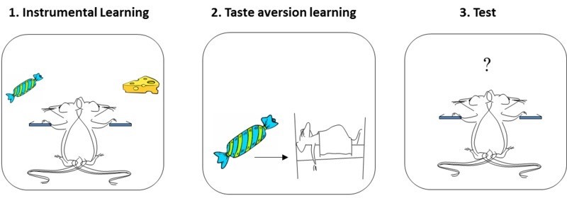
2. Habits are developed by overtraining Stimulus \rightarrow Response associations.

• The main difference is that habits are not influenced by outcome devaluation, i.e. when rewards lose their value.

Source: Bernard W. Balleine

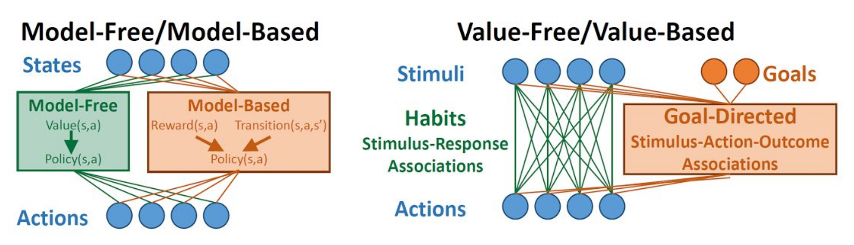
Goal-directed / habits = MB / MF ?

• The classical theory assigns MF to habits and MB to goal-directed, mostly because their sensitivity to outcome devaluation.

• The open question is the arbitration mechanism between these two segregated process: who takes control?

• Recent work suggests both systems are largely overlapping.

References

Doll, B. B., Simon, D. A., and Daw, N. D. (2012). The ubiquity of model-based reinforcement learning. Current Opinion in Neurobiology 22, 1075–1081. doi:10.1016/j.conb.2012.08.003.

Miller, K., Ludvig, E. A., Pezzulo, G., and Shenhav, A. (2018). “Re-aligning models of habitual and goal-directed decision-making,” in Goal-Directed Decision Making : Computations and Neural Circuits, eds. A. Bornstein, R. W. Morris, and A. Shenhav (Academic Press)

2 - Successor representations

Successor Representations (SR)

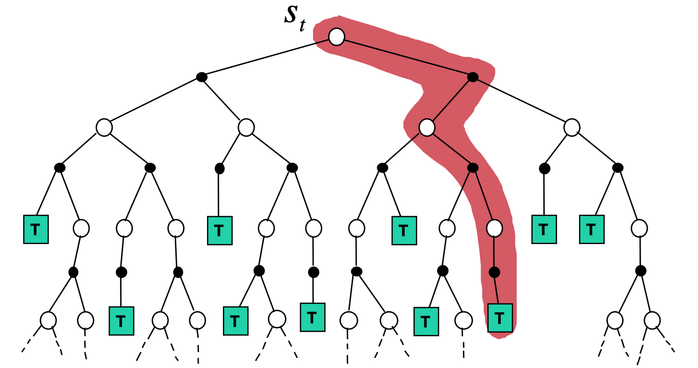
• Successor representations (SR) have been introduced to combine MF and MB properties. Let’s split the definition of the value of a state:

\begin{align} V^\pi(s) &= \mathbb{E}_{\pi} [\sum_{k=0}^\infty \gamma^k \, r_{t+k+1} | s_t =s] \\ &\\ &= \mathbb{E}_{\pi} [\begin{bmatrix} 1 \\ \gamma \\ \gamma^2 \\ \ldots \\ \gamma^\infty \end{bmatrix} \times \begin{bmatrix} \mathbb{I}(s_{t}) \\ \mathbb{I}(s_{t+1}) \\ \mathbb{I}(s_{t+2}) \\ \ldots \\ \mathbb{I}(s_{\infty}) \end{bmatrix} \times \begin{bmatrix} r_{t+1} \\ r_{t+2} \\ r_{t+3} \\ \ldots \\ r_{t+\infty} \end{bmatrix} | s_t =s]\\ \end{align}

where \mathbb{I}(s_{t}) is 1 when the agent is in s_t at time t, 0 otherwise.

• The left part corresponds to the transition dynamics: which states will be visited by the policy, discounted by \gamma.

• The right part corresponds to the immediate reward in each visited state.

• Couldn’t we learn the transition dynamics and the reward distribution separately in a model-free manner?

Successor Representations (SR)

• SR rewrites the value of a state into an expected discounted future state occupancy M^\pi(s, s') and an expected immediate reward r(s') by summing over all possible states s' of the MDP:

\begin{align} V^\pi(s) &= \mathbb{E}_{\pi} [\sum_{k=0}^\infty \gamma^k \, r_{t+k+1} | s_t =s] \\ &\\ &= \sum_{s' \in \mathcal{S}} \mathbb{E}_{\pi} [\sum_{k=0}^\infty \gamma^k \, \mathbb{I}(s_{t+k}=s') \times r_{t+k+1} | s_t =s]\\ &\\ &\approx \sum_{s' \in \mathcal{S}} \mathbb{E}_{\pi} [\sum_{k=0}^\infty \gamma^k \, \mathbb{I}(s_{t+k}=s') | s_t =s] \times \mathbb{E} [r_{t+1} | s_{t}=s']\\ &\\ &\approx \sum_{s' \in \mathcal{S}} M^\pi(s, s') \times r(s')\\ \end{align}

Successor Representations (SR)

• The underlying assumption is that the world dynamics are independent from the reward function (which does not depend on the policy).

• This allows to re-use knowledge about world dynamics in other contexts (e.g. a new reward function in the same environment): transfer learning.

Source: https://awjuliani.medium.com/the-present-in-terms-of-the-future-successor-representations-in-reinforcement-learning-316b78c5fa3

• What matters is the states that you will visit and how interesting they are, not the order in which you visit them.

• Knowing that being in the mensa will eventually get you some food is enough to know that being in the mensa is a good state: you do not need to remember which exact sequence of transitions will put food in your mouth.

Successor Representations (SR)

• SR algorithms must estimate two quantities:

  1. The expected immediate reward received after each state:

  r(s) = \mathbb{E} [r_{t+1} | s_t = s]

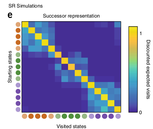
  2. The expected discounted future state occupancy (the SR itself):

  M^\pi(s, s') = \mathbb{E}_{\pi} [\sum_{k=0}^\infty \gamma^k \, \mathbb{I}(s_{t+k} = s') | s_t = s]

• The value of a state s is then computed with:

V^\pi(s) = \sum_{s' \in \mathcal{S}} M(s, s') \times r(s')

what allows to infer the policy (e.g. using an actor-critic architecture).

• The immediate reward for a state can be estimated very quickly and flexibly after receiving each reward:

\Delta \, r(s_t) = \alpha \, (r_{t+1} - r(s_t))

SR and transition matrix

• Imagine a very simple MDP with 4 states and a single deterministic action:

• The transition matrix \mathcal{P}^\pi depicts the possible (s, s') transitions:

\mathcal{P}^\pi = \begin{bmatrix} 0 & 1 & 0 & 0 \\ 0 & 0 & 1 & 0 \\ 0 & 0 & 0 & 1 \\ 0 & 0 & 0 & 1 \\ \end{bmatrix}

• The SR matrix M also represents the future transitions discounted by \gamma:

M = \begin{bmatrix} 1 & \gamma & \gamma^2 & \gamma^3 \\ 0 & 1 & \gamma & \gamma^2 \\ 0 & 0 & 1 & \gamma\\ 0 & 0 & 0 & 1 \\ \end{bmatrix}

SR matrix in a Tolman’s maze

• The SR represents whether a state can be reached soon from the current state (b) using the current policy.

• The SR depends on the policy:

  • A random agent will map the local neighborhood (c).

  • A goal-directed agent will have SR representations that follow the optimal path (d).

• It is therefore different from the transition matrix, as it depends on behavior and rewards.

• The exact dynamics are lost compared to MB: it only represents whether a state is reachable, not how.

Example of a SR matrix

• The SR matrix reflects the proximity between states depending on the transitions and the policy. it does not have to be a spatial relationship.

Learning the SR

• How can we learn the SR matrix for all pairs of states?

M^\pi(s, s') = \mathbb{E}_{\pi} [\sum_{k=0}^\infty \gamma^k \, \mathbb{I}(s_{t+k} = s') | s_t = s]

• We first notice that the SR obeys a recursive Bellman-like equation:

\begin{aligned} M^\pi(s, s') &= \mathbb{I}(s_{t} = s') + \mathbb{E}_{\pi} [\sum_{k=1}^\infty \gamma^k \, \mathbb{I}(s_{t+k} = s') | s_t = s] \\ &= \mathbb{I}(s_{t} = s') + \gamma \, \mathbb{E}_{\pi} [\sum_{k=0}^\infty \gamma^k \, \mathbb{I}(s_{t+k+1} = s') | s_t = s] \\ &= \mathbb{I}(s_{t} = s') + \gamma \, \mathbb{E}_{s_{t+1} \sim \mathcal{P}^\pi(s' | s)} [\mathbb{E}_{\pi} [\sum_{k=0}^\infty \gamma^k \, \mathbb{I}(s_{t+k} = s') | s_{t+1} = s] ]\\ &= \mathbb{I}(s_{t} = s') + \gamma \, \mathbb{E}_{s_{t+1} \sim \mathcal{P}^\pi(s' | s)} [M^\pi(s_{t+1}, s')]\\ \end{aligned}

• This is reminiscent of TDM: the remaining distance to the goal is 0 if I am already at the goal, or gamma the distance from the next state to the goal.

Model-based SR

• Bellman-like SR:

M^\pi(s, s') = \mathbb{I}(s_{t} = s') + \gamma \, \mathbb{E}_{s_{t+1} \sim \mathcal{P}^\pi(s' | s)} [M^\pi(s_{t+1}, s')]

• If we know the transition matrix for a fixed policy \pi:

\mathcal{P}^\pi(s, s') = \sum_a \pi(s, a) \, p(s' | s, a)

we can obtain the SR directly with matrix inversion as we did in dynamic programming:

M^\pi = I + \gamma \, \mathcal{P}^\pi \times M^\pi

so that:

M^\pi = (I - \gamma \, \mathcal{P}^\pi)^{-1}

• This DP approach is called model-based SR (MB-SR) as it necessitates to know the environment dynamics.

Model-free SR

• If we do not know the transition probabilities, we simply sample a single s_t, s_{t+1} transition:

M^\pi(s_t, s') \approx \mathbb{I}(s_{t} = s') + \gamma \, M^\pi(s_{t+1}, s')

• We can define a sensory prediction error (SPE):

\delta^\text{SR}_t = \mathbb{I}(s_{t} = s') + \gamma \, M^\pi(s_{t+1}, s') - M(s_t, s')

that is used to update an estimate of the SR:

\Delta M^\pi(s_t, s') = \alpha \, \delta^\text{SR}_t

• This is SR-TD, using a SPE instead of RPE, which learns only from transitions but ignores rewards.

The sensory prediction error - SPE

• The SPE has to be applied on ALL successor states s' after a transition (s_t, s_{t+1}):

M^\pi(s_t, \mathbf{s'}) = M^\pi(s_t, \mathbf{s'}) + \alpha \, (\mathbb{I}(s_{t}=\mathbf{s'}) + \gamma \, M^\pi(s_{t+1}, \mathbf{s'}) - M(s_t, \mathbf{s'}))

• Contrary to the RPE, the SPE is a vector of prediction errors, used to update one row of the SR matrix.

• The SPE tells how surprising a transition s_t \rightarrow s_{t+1} is for the SR.

Successor representations

• The SR matrix represents the expected discounted future state occupancy:

M^\pi(s, s') = \mathbb{E}_{\pi} [\sum_{k=0}^\infty \gamma^k \, \mathbb{I}(s_{t+k} = s') | s_t = s]

• It can be learned using a TD-like SPE from single transitions:

M^\pi(s_t, \mathbf{s'}) = M^\pi(s_t, \mathbf{s'}) + \alpha \, (\mathbb{I}(s_{t}=\mathbf{s'}) + \gamma \, M^\pi(s_{t+1}, \mathbf{s'}) - M(s_t, \mathbf{s'}))

• The immediate reward in each state can be learned independently from the policy:

\Delta \, r(s_t) = \alpha \, (r_{t+1} - r(s_t))

• The value V^\pi(s) of a state is obtained by summing of all successor states:

V^\pi(s) = \sum_{s' \in \mathcal{S}} M(s, s') \times r(s')

• This critic can be used to train an actor \pi_\theta using regular TD learning (e.g. A3C).

Successor representation of actions

• Note that it is straightforward to extend the idea of SR to state-action pairs:

M^\pi(s, a, s') = \mathbb{E}_{\pi} [\sum_{k=0}^\infty \gamma^k \, \mathbb{I}(s_{t+k} = s') | s_t = s, a_t = a]

allowing to estimate Q-values:

Q^\pi(s, a) = \sum_{s' \in \mathcal{S}} M(s, a, s') \times r(s')

using SARSA or Q-learning-like SPEs:

\delta^\text{SR}_t = \mathbb{I}(s_{t} = s') + \gamma \, M^\pi(s_{t+1}, a_{t+1}, s') - M(s_t, a_{t}, s')

depending on the choice of the next action a_{t+1} (on- or off-policy).

3 - Successor features

Successor features

• The SR matrix associates each state to all others (N\times N matrix):

  • curse of dimensionality.

  • only possible for discrete state spaces.

• A better idea is to describe each state s by a feature vector \phi(s) = [\phi_i(s)]_{i=1}^d with less dimensions than the number of states.

• This feature vector can be constructed (see the lecture on function approximation) or learned by an autoencoder (latent representation).

Source: http://www.jessicayung.com/the-successor-representation-1-generalising-between-states/

Successor features

• The successor feature representation (SFR) represents the discounted probability of observing a feature \phi_j after being in s.

Source: http://www.jessicayung.com/the-successor-representation-1-generalising-between-states/

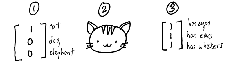
• Instead of predicting when the agent will see a cat after being in the current state s, the SFR predicts when it will see eyes, ears or whiskers independently:

M^\pi_j(s) = M^\pi(s, \phi_j) = \mathbb{E}_{\pi} [\sum_{k=0}^\infty \gamma^k \, \mathbb{I}(\phi_j(s_{t+k})) | s_t = s, a_t = a]

• Linear SFR (Gehring, 2015) supposes that it can be linearly approximated from the features of the current state:

M^\pi_j(s) = M^\pi(s, \phi_j) = \sum_{i=1}^d m_{i, j} \, \phi_i(s)

Successor features

• The value of a state is now defined as the sum over successor features of their immediate reward discounted by the SFR:

V^\pi(s) = \sum_{j=1}^d M^\pi_j(s) \, r(\phi_j) = \sum_{j=1}^d r(\phi_j) \, \sum_{i=1}^d m_{i, j} \, \phi_i(s)

• The SFR matrix M^\pi = [m_{i, j}]_{i, j} associates each feature \phi_i of the current state to all successor features \phi_j.

  • Knowing that I see a kitchen door in the current state, how likely will I see a food outcome in the near future?

• Each successor feature \phi_j is associated to an expected immediate reward r(\phi_j).

  • A good state is a state where food features (high r(\phi_j)) are likely to happen soon (high m_{i, j}).

• In matrix-vector form:

V^\pi(s) = \mathbf{r}^T \times M^\pi \times \phi(s)

Successor features

• Value of a state:

V^\pi(s) = \mathbf{r}^T \times M^\pi \times \phi(s)

• The reward vector \mathbf{r} only depends on the features and can be learned independently from the policy, but can be made context-dependent:

  • Food features can be made more important when the agent is hungry, less when thirsty.

• Transfer learning becomes possible in the same environment:

  • Different goals (searching for food or water, going to place A or B) only require different reward vectors.

  • The dynamics of the environment are stored in the SFR.

Source: https://awjuliani.medium.com/the-present-in-terms-of-the-future-successor-representations-in-reinforcement-learning-316b78c5fa3

Successor features

• How can we learn the SFR matrix M^\pi?

V^\pi(s) = \mathbf{r}^T \times M^\pi \times \phi(s)

• We only need to use the sensory prediction error for a transition between the feature vectors \phi(s_t) and \phi(s_{t+1}):

\delta_t^\text{SFR} = \phi(s_t) + \gamma \, M^\pi \times \phi(s_{t+1}) - M^\pi \times \phi(s_t)

and use it to update the whole matrix:

\Delta M^\pi = \delta_t^\text{SFR} \times \phi(s_t)^T

• However, this linear approximation scheme only works for fixed feature representation \phi(s). We need to go deeper…

4 - Deep Successor Reinforcement Learning

Deep Successor Reinforcement Learning

Deep Successor Reinforcement Learning

• Each state s_t is represented by a D-dimensional (D=512) vector \phi(s_t) = f_\theta(s_t) which is the output of an encoder.

• A decoder g_{\hat{\theta}} is used to provide a reconstruction loss, so \phi(s_t) is a latent representation of an autoencoder:

\mathcal{L}_\text{reconstruction}(\theta, \hat{\theta}) = \mathbb{E}[(g_{\hat{\theta}}(\phi(s_t)) - s_t)^2]

• The immediate reward R(s_t) is linearly predicted from the feature vector \phi(s_t) using a reward vector \mathbf{w}.

R(s_t) = \phi(s_t)^T \times \mathbf{w}

\mathcal{L}_\text{reward}(\mathbf{w}, \theta) = \mathbb{E}[(r_{t+1} - \phi(s_t)^T \times \mathbf{w})^2]

• The reconstruction loss is important, otherwise the latent representation \phi(s_t) would be too reward-oriented and would not generalize.

• The reward function is learned on a single task, but it can fine-tuned on another task, with all other weights frozen.

Deep Successor Reinforcement Learning

• For each action a, a NN u_\alpha predicts the future feature occupancy M(s, s', a) for the current state:

m_{s_t a} = u_\alpha(s_t, a)

• The Q-value of an action is simply the dot product between the SR of an action and the reward vector \mathbf{w}:

Q(s_t, a) = \mathbf{w}^T \times m_{s_t a}

• The selected action is \epsilon-greedily selected around the greedy action:

a_t = \text{arg}\max_a Q(s_t, a)

• The SR of each action is learned using the Q-learning-like SPE (with fixed \theta and a target network u_{\alpha'}):

\mathcal{L}^\text{SPE}(\alpha) = \mathbb{E}[\sum_a (\phi(s_t) + \gamma \, \max_{a'} u_{\alpha'}(s_{t+1}, a') - u_\alpha(s_t, a))^2]

• The compound loss is used to train the complete network end-to-end off-policy using a replay buffer (DQN-like).

\mathcal{L}(\theta, \hat{\theta}, \mathbf{w}, \alpha) = \mathcal{L}_\text{reconstruction}(\theta, \hat{\theta}) + \mathcal{L}_\text{reward}(\mathbf{w}, \theta) + \mathcal{L}^\text{SPE}(\alpha)

Deep Successor Reinforcement Learning

Deep Successor Reinforcement Learning

Deep Successor Reinforcement Learning

• The interesting property is that you do not need rewards to learn:

  • A random agent can be used to learn the encoder and the SR, but \mathbf{w} can be left untouched.

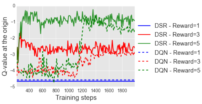
  • When rewards are introduced (or changed), only \mathbf{w} has to be adapted, while DQN would have to re-learn all Q-values.

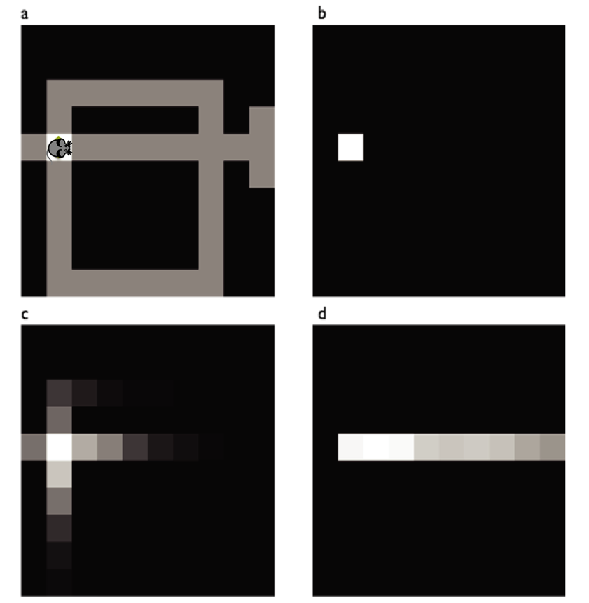
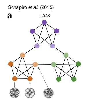
• This is the principle of latent learning in animal psychology: fooling around in an environment without a goal allows to learn the structure of the world, what can speed up learning when a task is introduced.

• The SR is a cognitive map of the environment: learning task-unspecific relationships.

Visual Semantic Planning using Deep Successor Representations

References

Dayan, P. (1993). Improving Generalization for Temporal Difference Learning: The Successor Representation. Neural Computation 5, 613–624. doi:10.1162/neco.1993.5.4.613.

Gehring, C. A. (2015). Approximate Linear Successor Representation. in, 5. http://people.csail.mit.edu/gehring/publications/clement-gehring-rldm-2015.pdf.

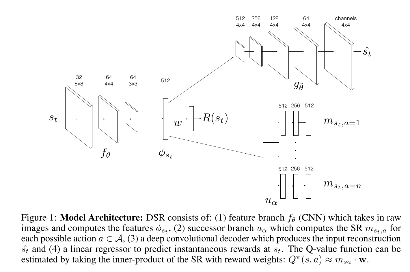
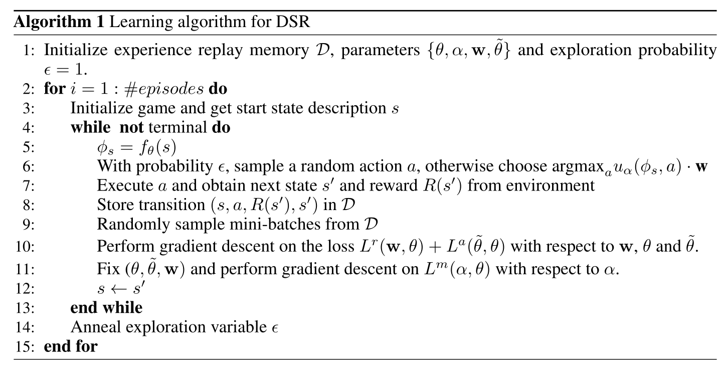
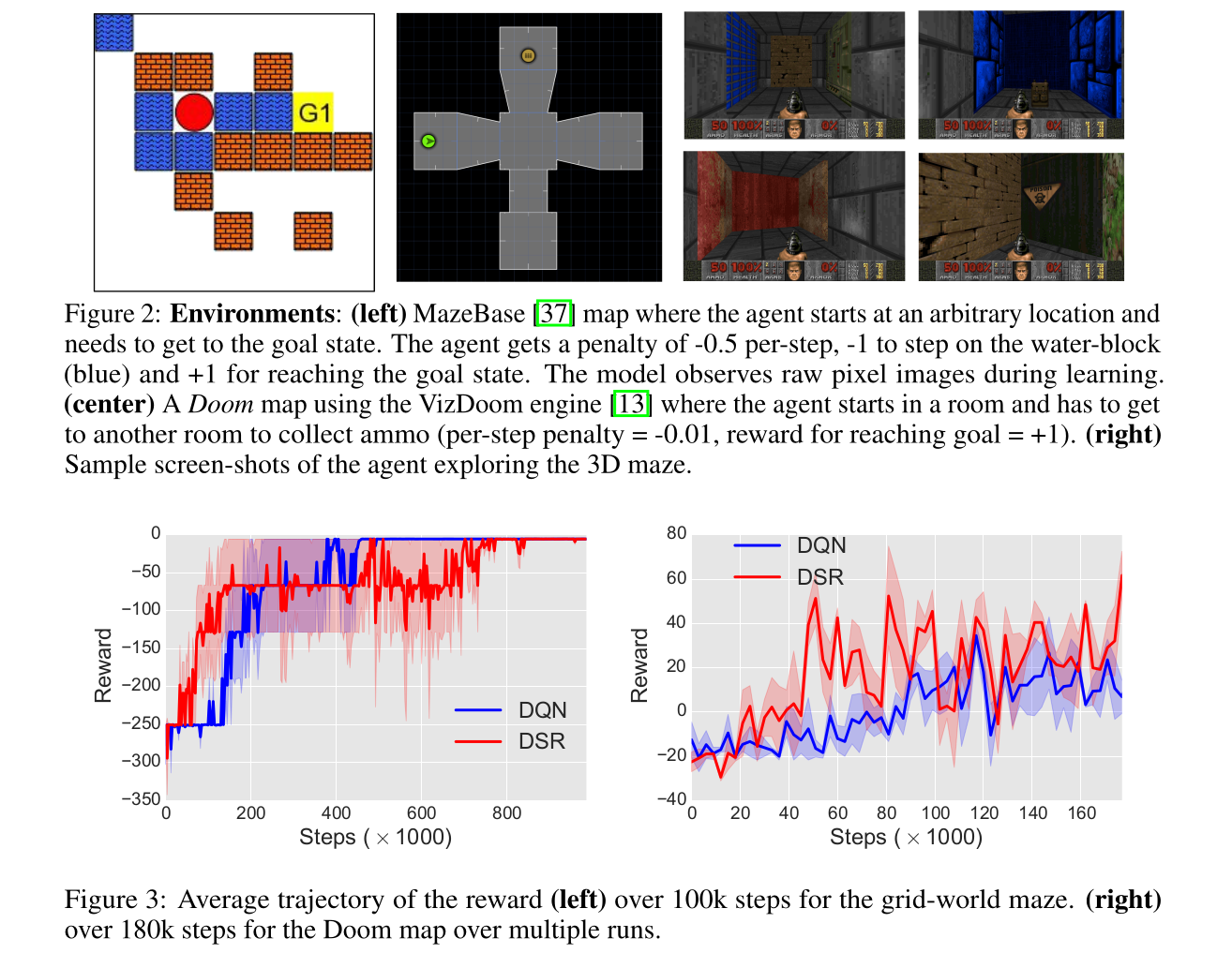
Kulkarni, T. D., Saeedi, A., Gautam, S., and Gershman, S. J. (2016). Deep Successor Reinforcement Learning. http://arxiv.org/abs/1606.02396.

Momennejad, I., Russek, E. M., Cheong, J. H., Botvinick, M. M., Daw, N. D., and Gershman, S. J. (2017). The successor representation in human reinforcement learning. Nature Human Behaviour 1, 680–692. doi:10.1038/s41562-017-0180-8.

Russek, E. M., Momennejad, I., Botvinick, M. M., Gershman, S. J., and Daw, N. D. (2017). Predictive representations can link model-based reinforcement learning to model-free mechanisms. PLOS Computational Biology 13, e1005768. doi:10.1371/journal.pcbi.1005768.

Stachenfeld, K. L., Botvinick, M. M., and Gershman, S. J. (2017). The hippocampus as a predictive map. Nature Neuroscience 20, 1643–1653. doi:10.1038/nn.4650.

Zhu, Y., Gordon, D., Kolve, E., Fox, D., Fei-Fei, L., Gupta, A., et al. (2017). Visual Semantic Planning using Deep Successor Representations. http://arxiv.org/abs/1705.08080.