Natural Language Processing and attention

Slides: html pdf

word2vec

The most famous application of RNNs is Natural Language Processing (NLP): text understanding, translation, etc… Each word of a sentence has to be represented as a vector \mathbf{x}_t in order to be fed to a LSTM. Which representation should we use?

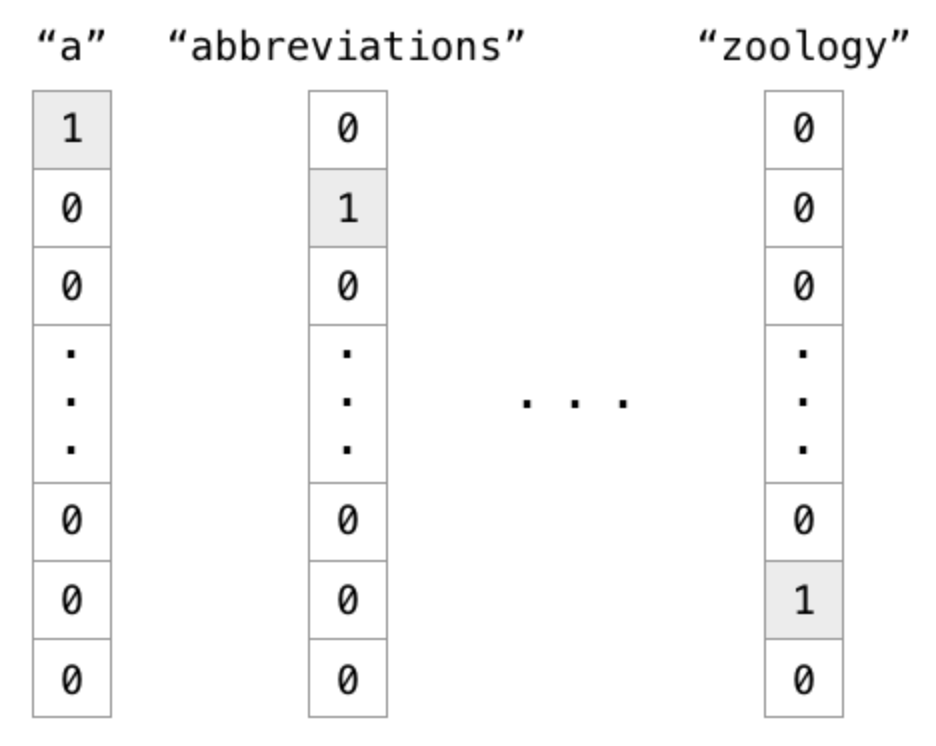
The naive solution is to use one-hot encoding, one element of the vector corresponding to one word of the dictionary.

One-hot encoding of words. Source: https://cdn-images-1.medium.com/max/1600/1*ULfyiWPKgWceCqyZeDTl0g.png.

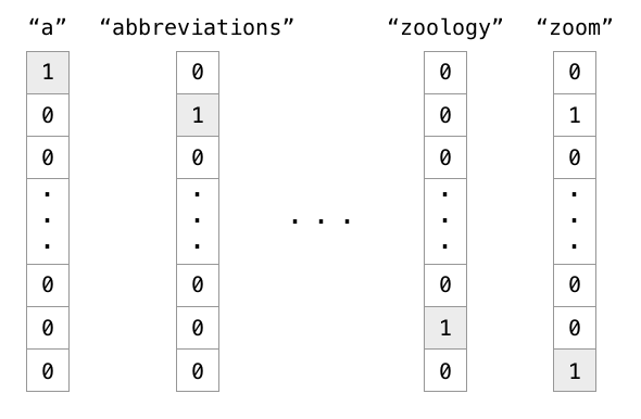
One-hot encoding is not a good representation for words:

• The vector size will depend on the number of words of the language:
  • English: 171,476 (Oxford English Dictionary), 470,000 (Merriam-Webster)… 20,000 in practice.
  • French: 270,000 (TILF).
  • German: 200,000 (Duden).
  • Chinese: 370,000 (Hanyu Da Cidian).
  • Korean: 1,100,373 (Woori Mal Saem)
• Semantically related words have completely different representations (“endure” and “tolerate”).
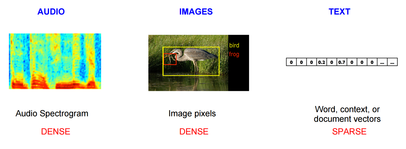
• The representation is extremely sparse (a lot of useless zeros).

Audio and image data are dense, i.e. each input dimension carries information. One-hot encoded sentences are sparse. Source: https://www.tensorflow.org/tutorials/representation/word2vec.

word2vec (Mikolov et al., 2013) learns word embeddings by trying to predict the current word based on the context (CBOW, continuous bag-of-words) or the context based on the current word (skip-gram). See https://code.google.com/archive/p/word2vec/ and https://www.tensorflow.org/tutorials/representation/word2vec for more information.

It uses a three-layer autoencoder-like NN, where the hidden layer (latent space) will learn to represent the one-hot encoded words in a dense manner.

Word2vec is an autoencoder trained to reproduce the context of a word using one-hot encoded vectors. Source: https://jaxenter.com/deep-learning-search-word2vec-147782.html.

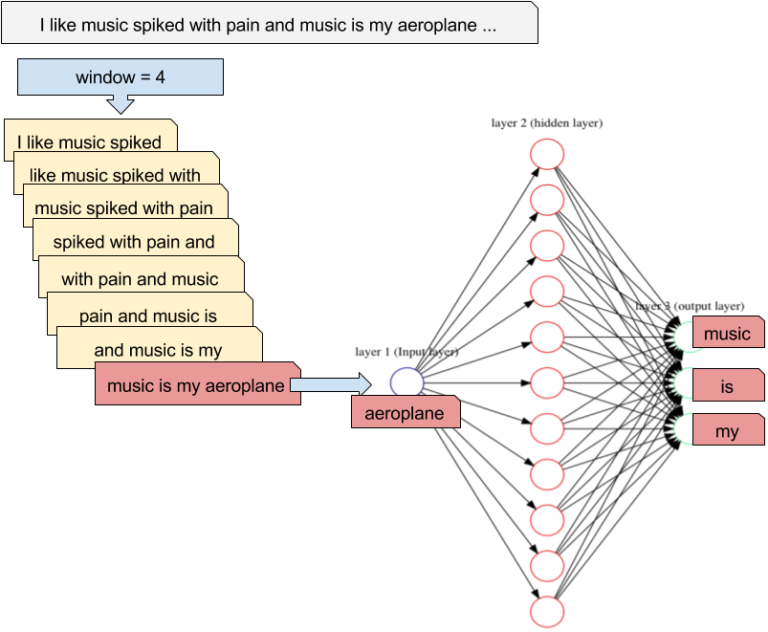
word2vec has three parameters:

• the vocabulary size: number of words in the dictionary.
• the embedding size: number of neurons in the hidden layer.
• the context size: number of surrounding words to predict.

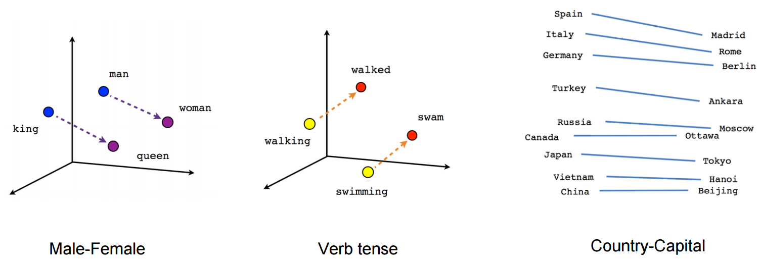
It is trained on huge datasets of sentences (e.g. Wikipedia). After learning, the hidden layer represents an embedding vector, which is a dense and compressed representation of each possible word (dimensionality reduction). Semantically close words (“endure” and “tolerate”) tend to appear in similar contexts, so their embedded representations will be close (Euclidian distance). One can even perform arithmetic operations on these vectors!

queen = king + woman - man

Arithmetic operations on word2vec representations. Source: https://www.tensorflow.org/tutorials/representation/word2vec.

Applications of RNNs

Classification of LSTM architectures

Several architectures are possible using recurrent neural networks:

Arithmetic operations on word2vec representations. Source: http://karpathy.github.io/2015/05/21/rnn-effectiveness/.

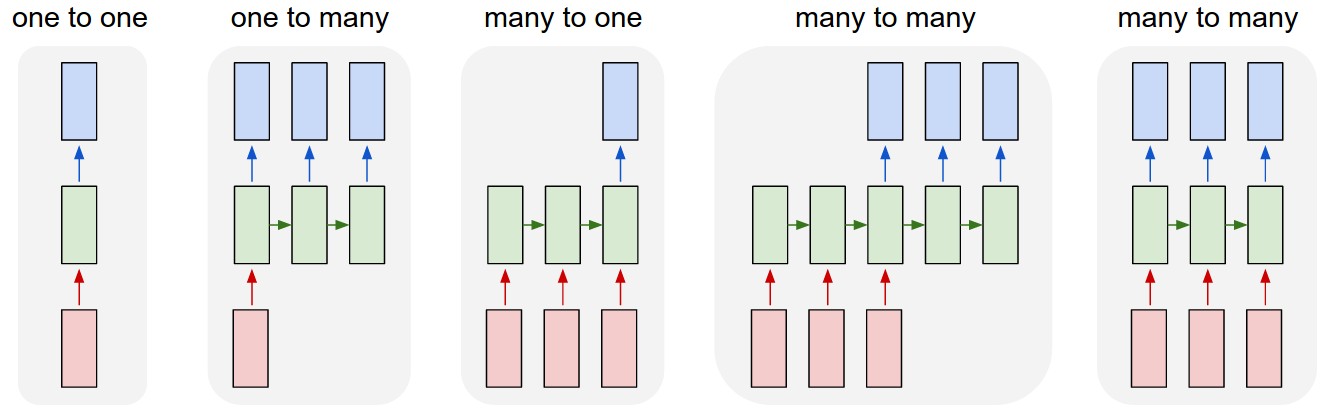
• One to One: classical feedforward network.
  • Image \rightarrow Label.
• One to Many: single input, many outputs.
  • Image \rightarrow Text.
• Many to One: sequence of inputs, single output.
  • Video / Text \rightarrow Label.
• Many to Many: sequence to sequence.
  • Text \rightarrow Text.
  • Video \rightarrow Text.

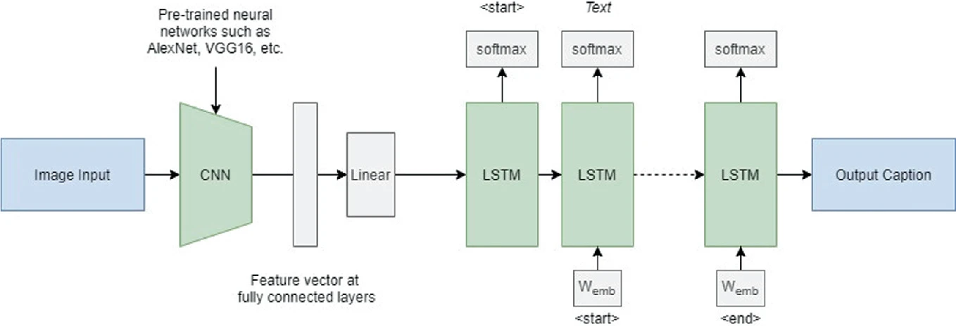
Image caption generation

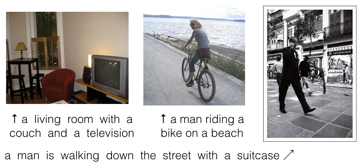
Show and Tell (Vinyals et al., 2015) uses the last FC layer of a CNN to feed a LSTM layer and generate words. The pretrained CNN (VGG16, ResNet50) is used as a feature extractor. Each word of the sentence is encoded/decoded using word2vec. The output of the LSTM at time t becomes its new input at time t+1.

Show and Tell architecture. Source: (Sathe et al., 2022).

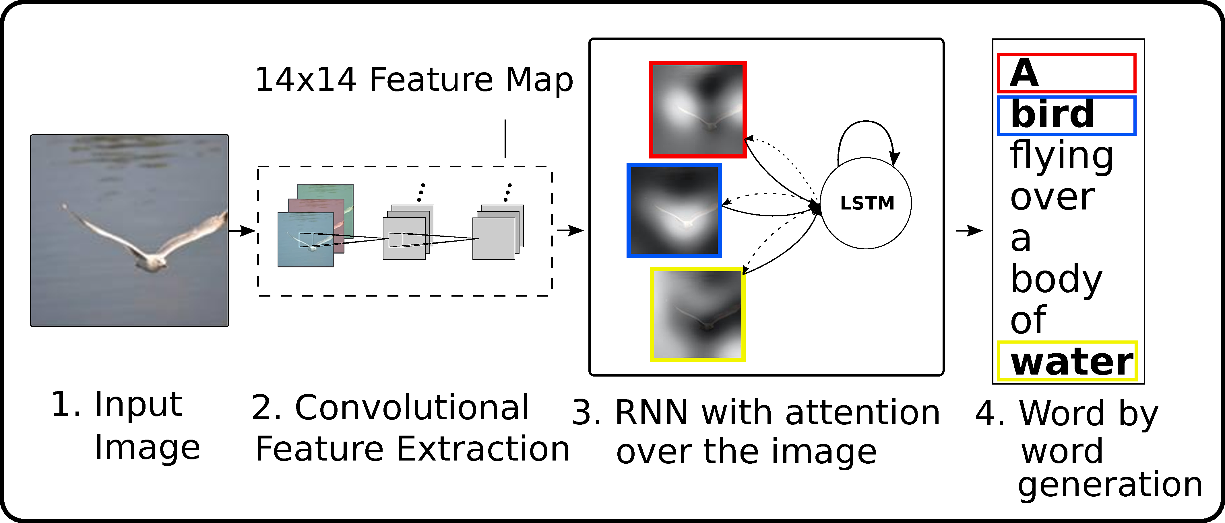
Show, attend and tell (Xu et al., 2015) uses attention to focus on specific parts of the image when generating the sentence.

Show, attend and tell (Xu et al., 2015).

Caption generation using Show, attend and tell (Xu et al., 2015).

Next character/word prediction

Characters or words are fed one by one into a LSTM. The desired output is the next character or word in the text.

Example:

• Inputs: To, be, or, not, to
• Output: be

The text below was generated by a LSTM having read the entire writings of William Shakespeare, learning to predict the next letter (see http://karpathy.github.io/2015/05/21/rnn-effectiveness/). Each generated character is used as the next input.

PANDARUS:
Alas, I think he shall be come approached and the day
When little srain would be attain'd into being never fed,
And who is but a chain and subjects of his death,
I should not sleep.

Second Senator:
They are away this miseries, produced upon my soul,
Breaking and strongly should be buried, when I perish
The earth and thoughts of many states.

DUKE VINCENTIO:
Well, your wit is in the care of side and that.

Second Lord:
They would be ruled after this chamber, and
my fair nues begun out of the fact, to be conveyed,
Whose noble souls I'll have the heart of the wars.

Clown:
Come, sir, I will make did behold your worship.

Sunspring SciFi movie

More info: http://www.thereforefilms.com/sunspring.html

Sentiment analysis

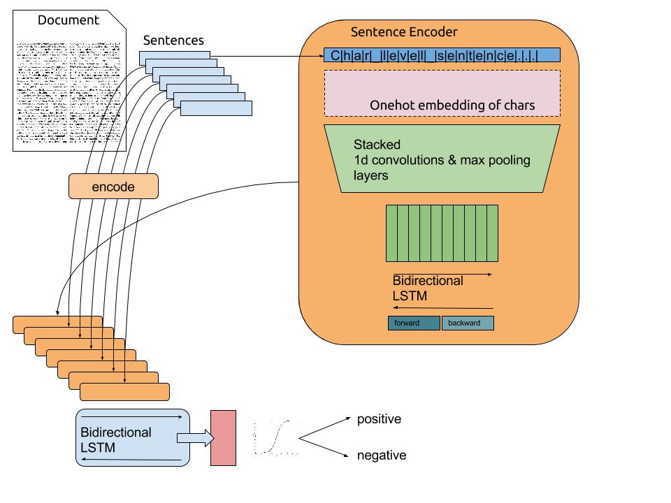
Sentiment analysis consists of attributing a value (positive or negative) to a text. A 1D convolutional layers “slides” over the text, each word being encoded using word2vec. The bidirectional LSTM computes a state vector for the complete text. A classifier (fully connected layer) learns to predict the sentiment of the text (positive/negative).

Sentiment analysis using bidirectional LSTMs. Source: https://offbit.github.io/how-to-read/.

Question answering / Scene understanding

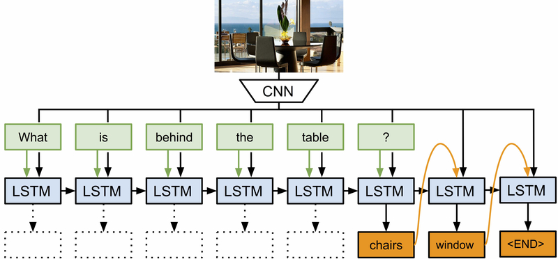
A LSTM can learn to associate an image (static) plus a question (sequence) with the answer (sequence). The image is abstracted by a CNN pretrained for object recognition.

Question answering. Source: (Malinowski et al., 2015).

seq2seq

The state vector obtained at the end of a sequence can be reused as an initial state for another LSTM. The goal of the encoder is to find a compressed representation of a sequence of inputs. The goal of the decoder is to generate a sequence from that representation. Sequence-to-sequence (seq2seq (Sutskever et al., 2014)) models are recurrent autoencoders.

seq2seq architecture. Source: (Sutskever et al., 2014).

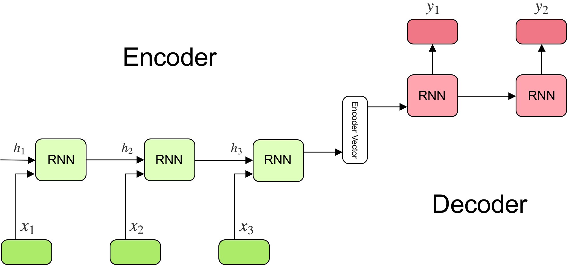
The encoder learns for example to encode each word of a sentence in French. The decoder learns to associate the final state vector to the corresponding English sentence. seq2seq allows automatic text translation between many languages given enough data. Modern translation tools are based on seq2seq, but with attention.

RNNs with Attention

Note

The videos in this section are taken from a great blog post by Jay Alammar:

https://jalammar.github.io/visualizing-neural-machine-translation-mechanics-of-seq2seq-models-with-attention/

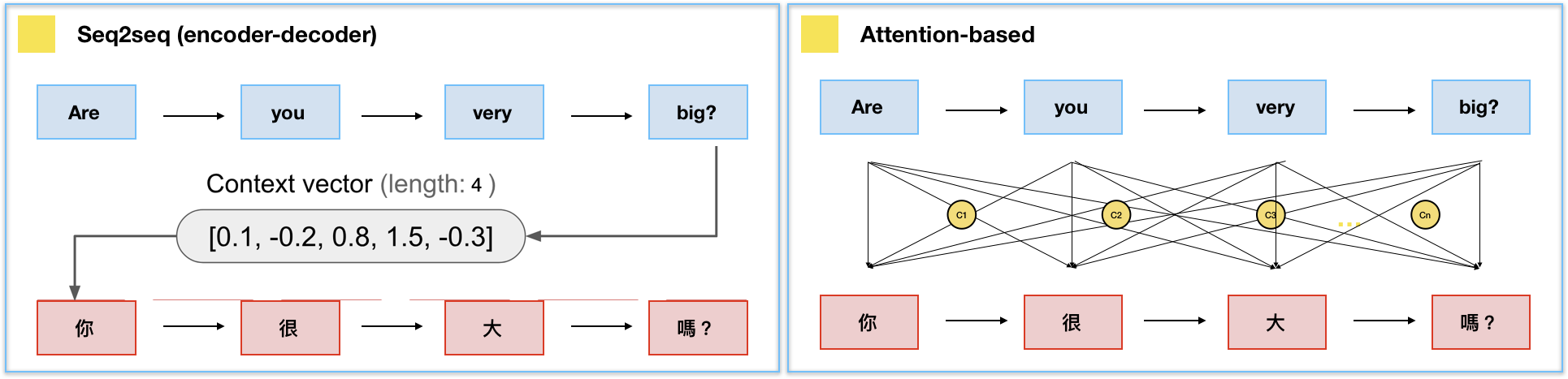
The problem with the seq2seq architecture is that it compresses the complete input sentence into a single state vector.

For long sequences, the beginning of the sentence may not be present in the final state vector:

• Truncated BPTT, vanishing gradients.
• When predicting the last word, the beginning of the paragraph might not be necessary.

Consequence: there is not enough information in the state vector to start translating. A solution would be to concatenate the state vectors of all steps of the encoder and pass them to the decoder.

• Problem 1: it would make a lot of elements in the state vector of the decoder (which should be constant).
• Problem 2: the state vector of the decoder would depend on the length of the input sequence.

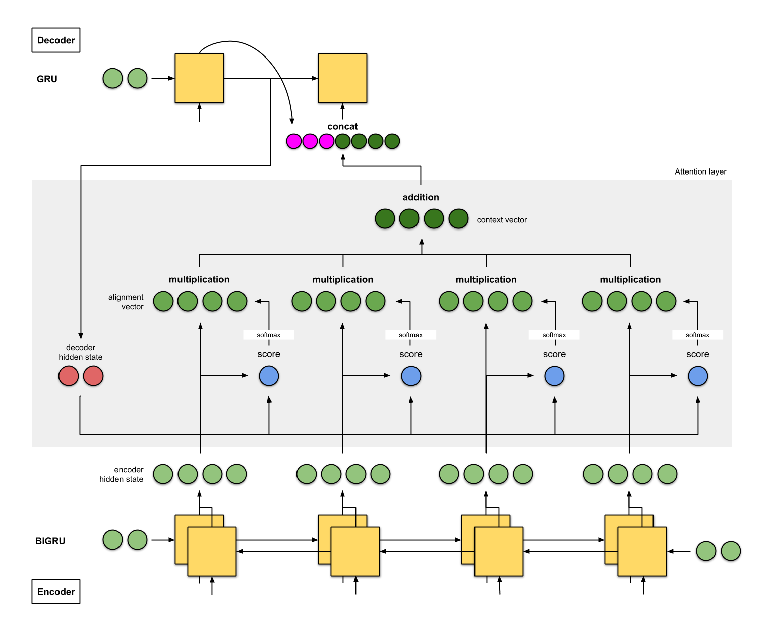
Attentional mechanisms (Bahdanau et al., 2016) let the decoder decide (by learning) which state vectors it needs to generate each word at each step.

The attentional context vector of the decoder A^\text{decoder}_t at time t is a weighted average of all state vectors C^\text{encoder}_i of the encoder.

A^\text{decoder}_t = \sum_{i=0}^T a_i \, C^\text{encoder}_i

The coefficients a_i are called the attention scores : how much attention is the decoder paying to each of the encoder’s state vectors? The attention scores a_i are computed as a softmax over the scores e_i (in order to sum to 1):

a_i = \frac{\exp e_i}{\sum_j \exp e_j} \Rightarrow A^\text{decoder}_t = \sum_{i=0}^T \frac{\exp e_i}{\sum_j \exp e_j} \, C^\text{encoder}_i

The score e_i is computed using:

• the previous output of the decoder \mathbf{h}^\text{decoder}_{t-1}.
• the corresponding state vector C^\text{encoder}_i of the encoder at step i.
• attentional weights W_a.

e_i = \text{tanh}(W_a \, [\mathbf{h}^\text{decoder}_{t-1}; C^\text{encoder}_i])

Everything is differentiable, these attentional weights can be learned with BPTT.

The attentional context vector A^\text{decoder}_t is concatenated with the previous output \mathbf{h}^\text{decoder}_{t-1} and used as the next input \mathbf{x}^\text{decoder}_t of the decoder:

\mathbf{x}^\text{decoder}_t = [\mathbf{h}^\text{decoder}_{t-1} ; A^\text{decoder}_t]

Seq2seq architecture with attention (Bahdanau et al., 2016). Source: https://towardsdatascience.com/day-1-2-attention-seq2seq-models-65df3f49e263.

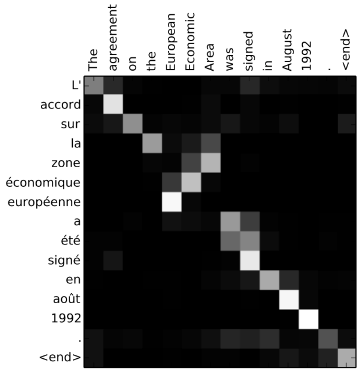
The attention scores or alignment scores a_i are useful to interpret what happened. They show which words in the original sentence are the most important to generate the next word.

Alignment scores during translation. Source: https://towardsdatascience.com/day-1-2-attention-seq2seq-models-65df3f49e263.

Attentional mechanisms are now central to NLP. The whole history of encoder states is passed to the decoder, which learns to decide which part is the most important using attention. This solves the bottleneck of seq2seq architectures, at the cost of much more operations. They require to use fixed-length sequences (generally 50 words).

Comparison of seq2seq and seq2seq with attention. Source: https://towardsdatascience.com/day-1-2-attention-seq2seq-models-65df3f49e263.

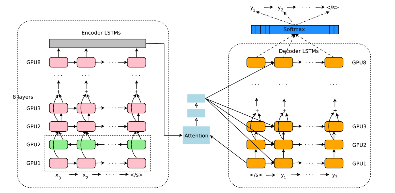
Google Neural Machine Translation (GNMT (Wu et al., 2016)) uses an attentional recurrent NN, with bidirectional GRUs, 8 recurrent layers on 8 GPUs for both the encoder and decoder.

Google Neural Machine Translation (GNMT (Wu et al., 2016))

Bahdanau, D., Cho, K., and Bengio, Y. (2016). Neural Machine Translation by Jointly Learning to Align and Translate. http://arxiv.org/abs/1409.0473.

Malinowski, M., Rohrbach, M., and Fritz, M. (2015). Ask Your Neurons: A Neural-based Approach to Answering Questions about Images. http://arxiv.org/abs/1505.01121.

Mikolov, T., Chen, K., Corrado, G., and Dean, J. (2013). Efficient Estimation of Word Representations in Vector Space. http://arxiv.org/abs/1301.3781.

Sathe, S., Shinde, S., Chorge, S., Thakare, S., and Kulkarni, L. (2022). Overview of Image Caption Generators and Its Applications. in Proceeding of International Conference on Computational Science and Applications Algorithms for Intelligent Systems., eds. S. Bhalla, M. Bedekar, R. Phalnikar, and S. Sirsikar (Singapore: Springer Nature), 105–110. doi:10.1007/978-981-19-0863-7_8.

Sutskever, I., Vinyals, O., and Le, Q. V. (2014). Sequence to Sequence Learning with Neural Networks. http://arxiv.org/abs/1409.3215.

Vinyals, O., Toshev, A., Bengio, S., and Erhan, D. (2015). Show and Tell: A Neural Image Caption Generator. http://arxiv.org/abs/1411.4555.

Wu, Y., Schuster, M., Chen, Z., Le, Q. V., Norouzi, M., Macherey, W., et al. (2016). Google’s Neural Machine Translation System: Bridging the Gap between Human and Machine Translation. https://arxiv.org/abs/1609.08144v2.

Xu, K., Ba, J. L., Kiros, R., Cho, K., Courville, A., Salakhutdinov, R., et al. (2015). Show, Attend and Tell: Neural Image Caption Generation with Visual Attention. in Proceedings of the 32nd International Conference on Machine Learning - Volume 37 ICML’15. (JMLR.org), 2048–2057. http://dl.acm.org/citation.cfm?id=3045118.3045336.