Neurocomputing

Optimization

Julien Vitay

Professur für Künstliche Intelligenz - Fakultät für Informatik

1 - Optimization

Machine learning = Optimization

Machine learning is all about optimization:
- Supervised learning minimizes the error between the prediction and the data.
- Unsupervised learning maximizes the fit between the model and the data
- Reinforcement learning maximizes the collection of rewards.

The function to be optimized is called the objective function, cost function or loss function.
ML searches for the value of free parameters which optimize the objective function on the data set.
The simplest optimization method is the gradient descent (or ascent) method.

Analytical optimization

The easiest method to find the extremum of a function f(x) is to look where its first derivative is equal to 0:

x^* = \min_x f(x) \Leftrightarrow f'(x^*) = 0 \; \text{and} \; f''(x^*) > 0

x^* = \max_x f(x) \Leftrightarrow f'(x^*) = 0 \; \text{and} \; f''(x^*) < 0

The sign of the second order derivative tells us whether it is a maximum or minimum.

There can be multiple minima or maxima (or none) depending on the function.
- The “best” minimum (with the lowest value among all minima) is called the global minimum.
- The others are called local minima.

Multivariate optimization

A multivariate function is a function of more than one variable, e.g. f(x, y).

A point (x^*, y^*) is an extremum of f if all partial derivatives are zero at the same time:

\begin{cases} \dfrac{\partial f(x^*, y^*)}{\partial x} = 0 \\ \\ \dfrac{\partial f(x^*, y^*)}{\partial y} = 0 \\ \end{cases}

The vector of partial derivatives is called the gradient of the function:

\nabla_{x, y} \, f(x, y) = \begin{bmatrix} \dfrac{\partial f(x, y)}{\partial x} \\ \\ \dfrac{\partial f(x, y)}{\partial y} \end{bmatrix}

Finding the extremum of f is searching for the values of (x, y) where the gradient of the function is the zero vector:

\nabla_{x, y} \, f(x^*, y^*) = \begin{bmatrix} 0 \\ 0 \end{bmatrix}

Multivariate optimization : example

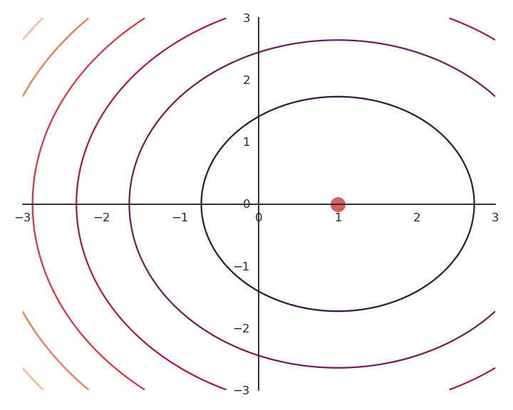
Let’s consider this function:

f(x, y) = (x - 1)^2 + y^2 + 1

Its gradient is:

\nabla_{x, y} \, f(x, y) = \begin{bmatrix} 2 (x -1) \\ 2 y \end{bmatrix}

The gradient is equal to 0 when:

\begin{cases} 2 \, (x -1) = 0 \\ 2 \, y = 0 \\ \end{cases}

\begin{bmatrix} 1 \\ 0 \end{bmatrix} is the minimum of f.

One should check the second order derivative to know whether it is a minimum or maximum…

2 - Gradient descent

Problem with analytical optimization

In machine learning, we generally do not have access to the analytical form of the objective function.
We can not therefore get its derivative and search where it is 0.
However, we have access to its value (and derivative) for certain values, for example:

f(0, 1) = 2 \qquad f'(0, 1) = -1.5

We can “ask” the model for as many values as we want, but we never get its analytical form.
For most useful problems, the function would be too complex to differentiate anyway.

Euler method

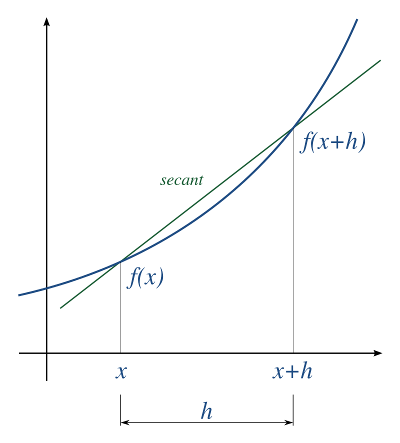
Let’s remember the definition of the derivative of a function. The derivative f'(x) is defined by the slope of the tangent of the function:

\begin{aligned} f'(x) & = \lim_{h \to 0} \frac{f(x + h) - f(x)}{x + h - x} \\ &\\ &= \lim_{h \to 0} \frac{f(x + h) - f(x)}{h} \\ \end{aligned}

If we take h small enough, we have the following approximation:

f(x + h) - f(x) \approx h \, f'(x)

We are making an error, but it is negligible if h is small enough (Taylor series).

Euler method

First order approximation:

f(x + h) - f(x) \approx h \, f'(x)

If we want x+h to be closer to the minimum than x, we want:

f(x + h) < f(x)

We therefore want that:

h \, f'(x) < 0

The change h in the value of x must have the opposite sign of f'(x).
- If the function is increasing in x, the minimum is smaller than x.
- If the function is decreasing in x, the minimum is bigger than x.

Gradient descent

Gradient descent (GD) is a first-order method to iteratively find the minimum of a function f(x).

It creates a series of estimates [x_0, x_1, x_2, \ldots] that converges to a local minimum of f.
Each element of the series is calculated based on the previous element and the derivative of the function in that element:

x_{n+1} = x_n + \Delta x = x_n - \eta \, f'(x_n)

\eta is a small parameter between 0 and 1 called the learning rate.

Gradient descent

Gradient descent algorithm

We start with an initially wrong estimate of x: x_0
for n \in [0, \infty]:
- We compute or estimate the derivative of the loss function in x_{n}: f'(x_{n})
- We compute a new value x_{n+1} for the estimate using the gradient descent update rule:
\Delta x = x_{n+1} - x_n = - \eta \, f'(x_n)

There is theoretically no end to the GD algorithm: we iterate forever and always get closer to the minimum.
The algorithm can be stopped when the change \Delta x is below a threshold.

Gradient descent

Multivariate gradient descent

Gradient descent can be applied to multivariate functions:

\min_{x, y, z} \qquad f(x, y, z)

Each variable is updated independently using partial derivatives:

\Delta x = x_{n+1} - x_{n} = - \eta \, \frac{\partial f(x_n, y_n, z_n)}{\partial x} \Delta y = y_{n+1} - y_{n} = - \eta \, \frac{\partial f(x_n, y_n, z_n)}{\partial y} \Delta z = z_{n+1} - z_{n} = - \eta \, \frac{\partial f(x_n, y_n, z_n)}{\partial z}

We can also use the vector notation to use the gradient operator:

\mathbf{x}_n = \begin{bmatrix} x_n \\ y_n \\ z_n \end{bmatrix} \quad \text{and} \quad \nabla_\mathbf{x} \, f(\mathbf{x}) = \begin{bmatrix} \dfrac{\partial f(x, y, z)}{\partial x} \\ \\ \dfrac{\partial f(x, y, z)}{\partial y} \\ \\ \dfrac{\partial f(x, y, z)}{\partial z} \end{bmatrix}

which gives:

\Delta \mathbf{x} = - \eta \, \nabla_\mathbf{x} \, f(\mathbf{x}_n)

Multivariate gradient descent

Influence of the learning rate

The parameter \eta is called the learning rate (or step size) and regulates the speed of convergence.
The choice of the learning rate \eta is critical:
- If it is too small, the algorithm will need a lot of iterations to converge.
- If it is too big, the algorithm can oscillate around the desired values without ever converging.

Optimality of gradient descent

Gradient descent is not optimal: it always finds a local minimum, but there is no guarantee that it is the global minimum.
The found solution depends on the initial choice of x_0. If you initialize the parameters near to the global minimum, you are lucky. But how?
This will be a big issue in neural networks.

3 - Regularization

Regularization

Most of the time, there are many minima to a function, if not an infinity.
As GD only converges to the “closest” local minimum, you are never sure that you get a good solution.
Consider the following function:

f(x, y) = (x -1)^2

As it does not depend on y, whatever initial value y_0 will be considered as a solution.
As we will see later, this is something we do not want.

Regularization

L2 - Regularization

We may want to put the additional constraint that x and y should be as small as possible.
One possibility is to also minimize the Euclidian norm (or L2-norm) of the vector \mathbf{x} = [x, y].

\min_{x, y} ||\mathbf{x}||^2 = x^2 + y^2

Note that this objective is in contradiction with the original objective: (0, 0) minimizes the norm, but not the function f(x, y).
We construct a new function as the sum of f(x, y) and the norm of \mathbf{x}, weighted by the regularization parameter \lambda:

\mathcal{L}(x, y) = f(x, y) + \lambda \, (x^2 + y^2)

L2 - Regularization

For a fixed value of \lambda, for example 0.1, we now minimize using gradient descent the following loss function function:

\mathcal{L}(x, y) = f(x, y) + \lambda \, (x^2 + y^2)

We just need to compute its gradient:

\nabla_{x, y} \, \mathcal{L}(x, y) = \begin{bmatrix} \dfrac{\partial f(x, y)}{\partial x} + 2\, \lambda \, x \\ \\ \dfrac{\partial f(x, y)}{\partial y} + 2\, \lambda \, y \end{bmatrix}

and apply gradient descent iteratively:

\Delta \begin{bmatrix} x \\ y \end{bmatrix} = - \eta \, \nabla_{x, y} \, \mathcal{L}(x, y) = - \eta \, \begin{bmatrix} \dfrac{\partial f(x, y)}{\partial x} + 2\, \lambda \, x \\ \\ \dfrac{\partial f(x, y)}{\partial y} + 2\, \lambda \, y \end{bmatrix}

L2 - Regularization

You may notice that the result of the optimization is a bit off, it is not exactly (1, 0).
This is because we do not optimize f(x, y) directly, but \mathcal{L}(x, y).
Let’s look at the real landscape of the function.

\mathcal{L}(x, y) = f(x, y) + \lambda \, (x^2 + y^2)

L2 - Regularization

The optimization with GD works, it is just that the function is different.
The constraint on the Euclidian norm “attracts” or “distorts” the function towards (0, 0).
This may seem counter-intuitive, but we will see with deep networks that we can live with it.
Let’s now look at what happens when we increase \lambda (to 5.0).

L2 - Regularization

Now the result of the optimization is totally wrong: the constraint on the norm completely dominates the optimization process.

\mathcal{L}(x, y) = f(x, y) + \lambda \, (x^2 + y^2)

\lambda controls which of the two objectives, f(x, y) or x^2 + y^2, has the priority:
- When \lambda is small, f(x, y) dominates and the norm of \mathbf{x} can be anything.
- When \lambda is big, x^2 + y^2 dominates, the result will be very small but f(x, y) will have any value.
The right value for \lambda is hard to find. We will see later methods to experimentally find its most adequate value.

L1 - Regularization

Another form of regularization is L1 - regularization using the L1-norm (absolute values):

\mathcal{L}(x, y) = f(x, y) + \lambda \, (|x| + |y|)

Its gradient only depend on the sign of x and y:

\nabla_{x, y} \, \mathcal{L}(x, y) = \begin{bmatrix} \dfrac{\partial f(x, y)}{\partial x} + \lambda \, \text{sign}(x) \\ \\ \dfrac{\partial f(x, y)}{\partial y} + \lambda \, \text{sign}(y) \end{bmatrix}

It tends to lead to sparser value of (x, y), i.e. either x or y will be 0.