As the training set is finite and the samples i.i.d (independent and identically distributed), we can simply replace the expectation by a sampling average:
\mathcal{L}(w, b) = \frac{1}{N} \, \sum_{i=1}^{N} (t_i - y_i )^2
Linear regression
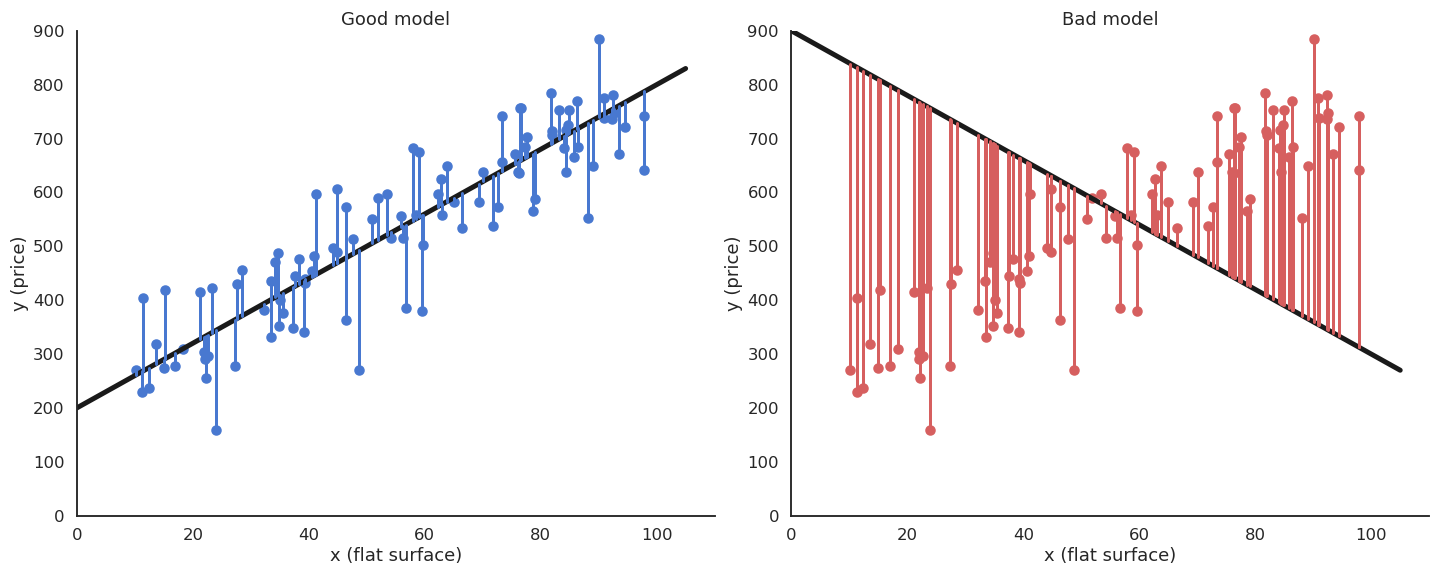
The minimum of the mse is achieved when the predictiony_i = f_{w, b}(x_i) is equal to the ground trutht_i for all training examples.
In other words, we want to minimize the residual error of the model on the data.
It is not always possible to obtain the global minimum (0) but the closer, the better.
Gradient descent for linear regression
We search for w and b which minimize the mean square error:
\mathcal{L}(w, b) = \frac{1}{N} \, \sum_{i=1}^{N} (t_i - y_i )^2
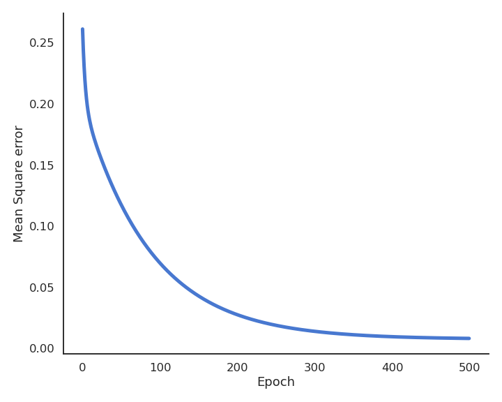
We will apply gradient descent to iteratively modify estimates of w and b:
\Delta w = - \eta \, \frac{\partial \mathcal{L}(w, b)}{\partial w}
\Delta b = - \eta \, \frac{\partial \mathcal{L}(w, b)}{\partial b}
Gradient descent for linear regression
Let’s search for the partial derivative (gradient) of the quadratic error with respect to w:
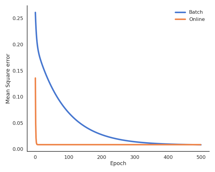
The batch version is more stable, but the online version is faster: the weights have already learned something when arriving at the end of the first epoch.
Delta learning rule in action (same learning rate!)
Delta learning rule
2 - Multiple linear regression
Multiple linear regression
The key idea of linear regression (one input x, one output y) can be generalized to multiple inputs and outputs.
Multiple Linear Regression (MLR) predicts several output variables based on several explanatory variables or features:
\begin{cases}
y_1 = w_1 \, x_1 + w_2 \, x_2 + b_1\\
\\
y_2 = w_3 \, x_1 + w_4 \, x_2 + b_2\\
\end{cases}
All we have is some samples: we want to know the best model for the data.
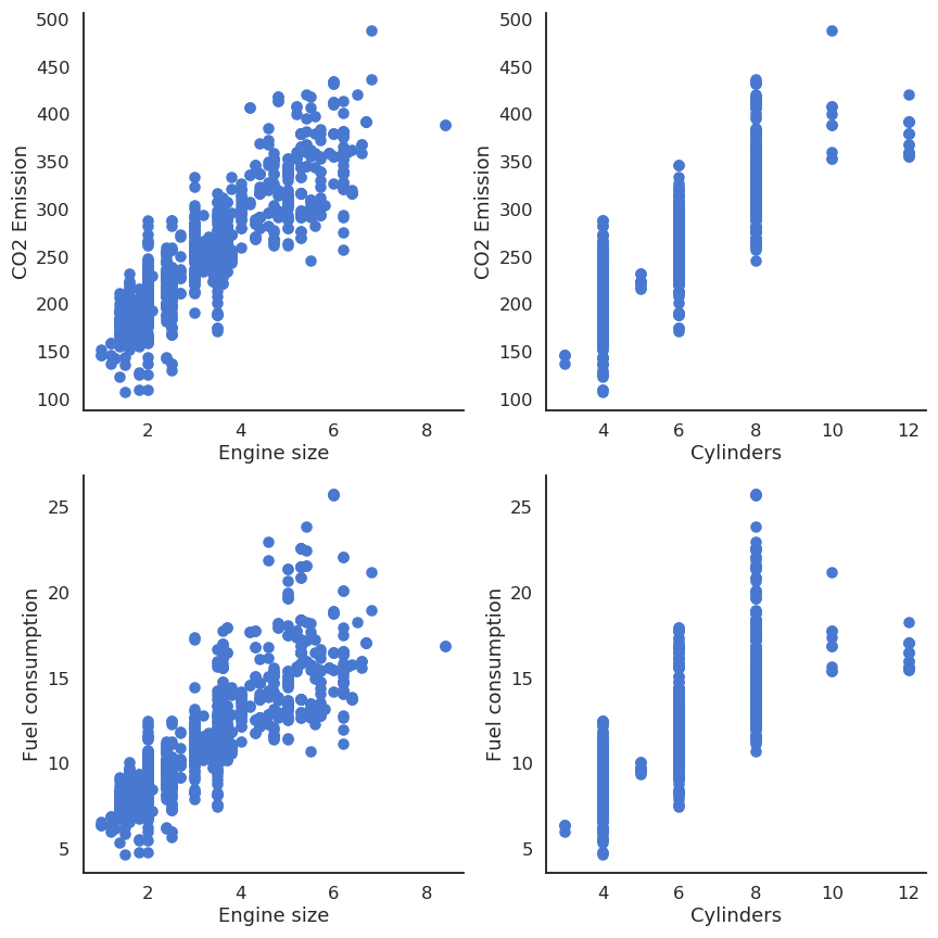
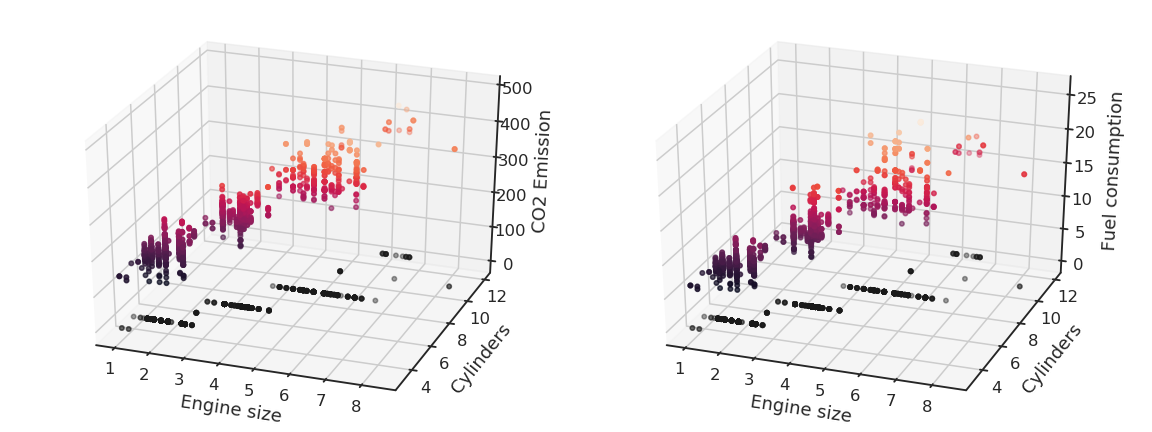
MLR example: fuel consumption and CO2 emissions
Let’s suppose you have 13971 measurements in some Excel file, linking engine size, number of cylinders, fuel consumption and CO2 emissions of various cars.
You want to predict fuel consumption and CO2 emissions when you know the engine size and the number of cylinders.
Engine size
Cylinders
Fuel consumption
CO2 emissions
2
4
8.5
196
2.4
4
9.6
221
1.5
4
5.9
136
3.5
6
11
255
3.5
6
11
244
3.5
6
10
230
3.5
6
10
232
3.7
6
11
255
3.7
6
12
267
…
…
…
…
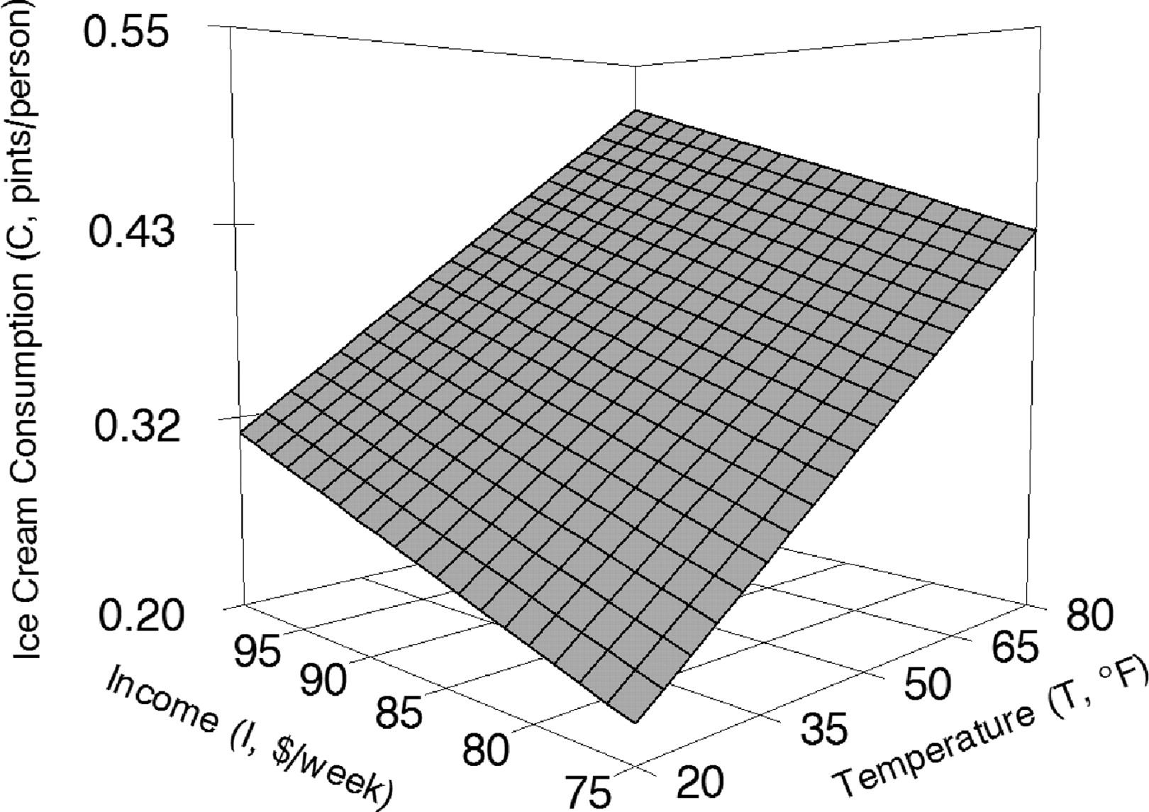
MLR example: fuel consumption and CO2 emissions
MLR example: fuel consumption and CO2 emissions
MLR example: fuel consumption and CO2 emissions
Noting the variables x_1, x_2, y_1, y_2, we can define our MLR problem:
\mathbf{x} is the input vector, \mathbf{y} is the output vector, \mathbf{t} is the target vector.
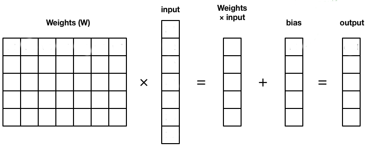
W is called the weight matrix and \mathbf{b} the bias vector.
\mathbf{y} = f_{W, \mathbf{b}}(\mathbf{x}) = W \times \mathbf{x} + \mathbf{b}
Multiple linear regression
The model is now defined by:
\mathbf{y} = f_{W, \mathbf{b}}(\mathbf{x}) = W \times \mathbf{x} + \mathbf{b}
The problem is exactly the same as before, except that we use vectors and matrices instead of scalars: \mathbf{x} and \mathbf{y} can have any number of dimensions, the same procedure will apply.
This corresponds to a linear neural network (or linear perceptron), with one output neuron per predicted value y_i using the linear activation function.
Multiple linear regression
The mean square error still needs to be a scalar in order to be minimized. We can define it as the squared norm of the error vector:
In order to apply gradient descent, one needs to calculate partial derivatives w.r.t the weight matrix W and the bias vector \mathbf{b}, i.e. gradients:
The individual loss function \mathcal{l}_i(W, \mathbf{b}) is the squared \mathcal{L}^2-norm of the error vector, what can be expressed as a dot product or a vector multiplication:
Note: We use the properties \nabla_{\mathbf{x}}\, \mathbf{x}^T \times \mathbf{z} = \mathbf{z} and \nabla_{\mathbf{z}} \, \mathbf{x}^T \times \mathbf{z} = \mathbf{x} to get rid of the transpose.
Multiple linear regression
The “problem” is when computing \nabla_{W} \, \mathbf{y}_i = \nabla_{W} \, (W \times \mathbf{x}_i + \mathbf{b}):
\mathbf{y}_i is a vector and W a matrix.
\nabla_{W} \, \mathbf{y}_i is then a Jacobian (matrix), not a gradient (vector).
Intuitively, differentiating W \times \mathbf{x}_i + \mathbf{b} w.r.t W should return \mathbf{x}_i, but it is a vector, not a matrix…
The gradient (or Jacobian) of \mathcal{l}_i(W, \mathbf{b}) w.r.t W should be a matrix of the same size as W so that we can apply gradient descent:
\Delta W = - \eta \, \nabla_W \, \mathcal{L}(W, \mathbf{b})
Non-linear problem solved! The only unknown is which order for the polynomial matches best the data.
One can perform regression with any kind of parameterized function using gradient descent.
5 - A bit of learning theory
What matters during training?
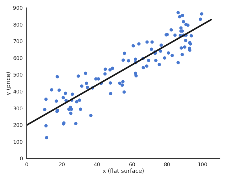
Before going further, let’s think about what we have been doing so far. We had a bunch of data samples \mathcal{D} = (x_i, t_i)_{i=1..N} (the training set) and we decided to apply a (linear) model on it:
y_i = w \, x_i + b
We then minimized the mean square error (mse) on that training set using gradient descent. At the end of learning, we can measure the residual error of the model on the data:
If you multiply both the data t and the prediction y by 10, the residual error will be 100 times higher, without any change to the quality of the model.
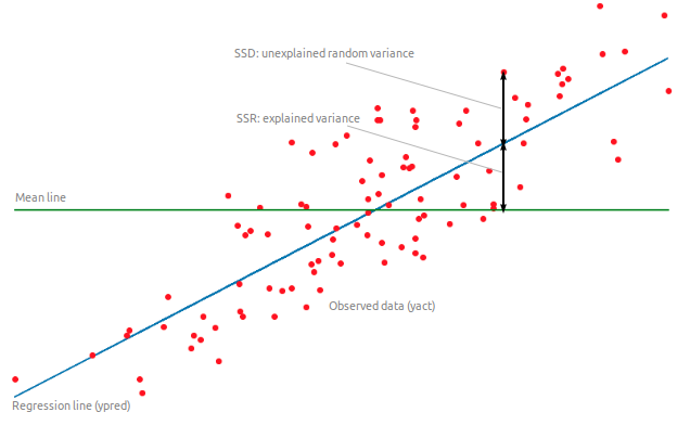
Coefficient of determination
The coefficient of determinationR^2 is a rescaled variant of the mse comparing the variance of the residuals to the variance of the data around its mean \hat{t}:
R^2 should be as close from 1 as possible. For example, if R^2 = 0.8, we can say that the model explains 80% of the variance of the data.
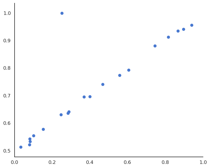
Sensibility to outliers
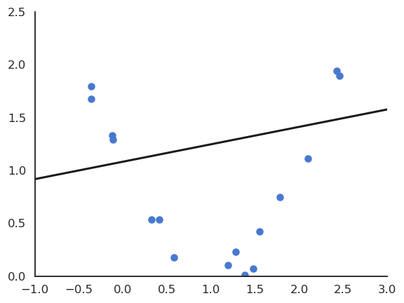
Suppose we have a training set with one outlier (bad measurement, bad luck, etc).
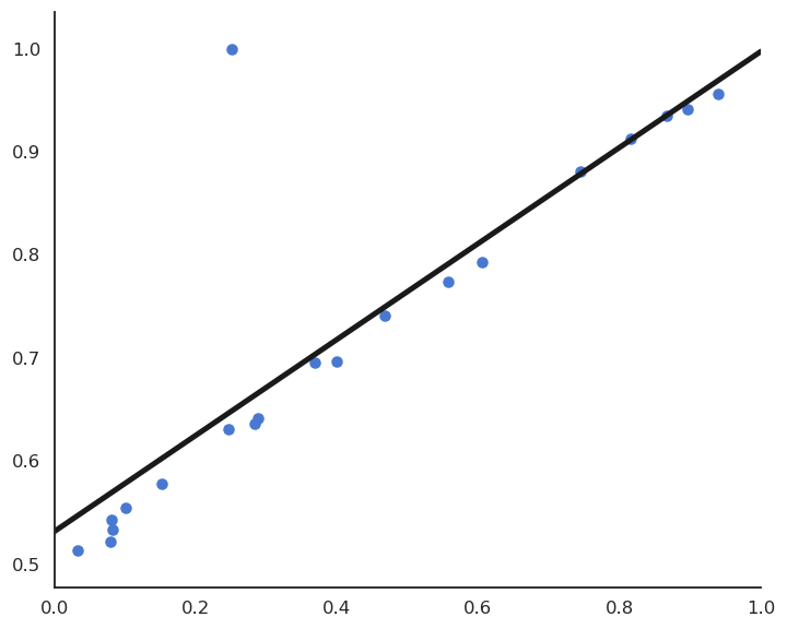
Sensibility to outliers
LMS would find the minimum of the mse, but it is clearly a bad fit for most points.
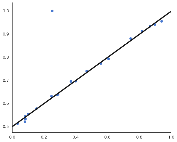
Sensibility to outliers
This model feels much better, but its residual mse is higher…
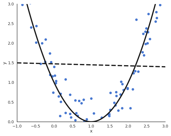
Polynomial regression
Polynomial regression
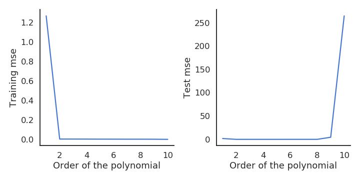
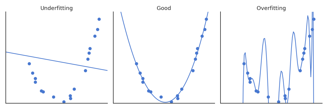
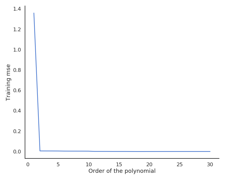
When only looking at the residual mse on the training data, one could think that the higher the order of the polynomial, the better.
But it is obvious that the interpolation quickly becomes very bad when the order is too high.
A complex model (with a lot of parameters) is useless for predicting new values.
We actually do not care about the error on the training set.
We care about generalization.
Cross-validation
Let’s suppose we dispose of m models \mathcal{M} = \{ M_1, ..., M_m\} that could be used to fit (or classify) some data \mathcal{D} = \{x_i, t_i\}_{i=1}^N.
Such a class could be the ensemble of polynomes with different orders, different algorithms (NN, SVM) or the same algorithm with different values for the hyperparameters (learning rate, regularization parameters…).
The naive and wrong method to find the best hypothesis would be:
Wrong method!
For all models M_i:
Train M_i on \mathcal{D} to obtain an hypothesis h_i.
Compute the training error \epsilon_\mathcal{D}(h_i) of h_i on \mathcal{D} :
Select the model M_{i}^* with the minimal empirical error on \mathcal{D}.
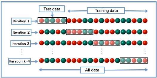
In general k=10. Extreme cases take k=N: leave-one-out cross-validation.
k-fold cross-validation works well, but needs a lot of repeated learning.
Validation data
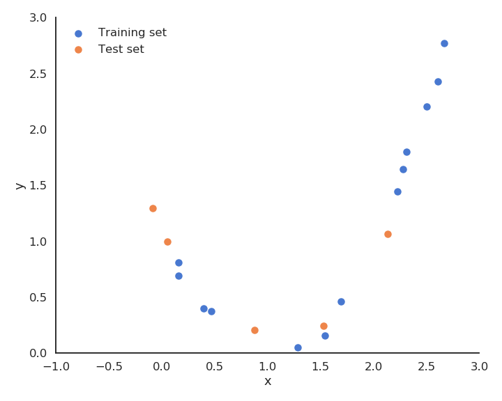
The bare minimum in ML is to have separate training and test sets. However, the test set should only be used once:
If you try many variations of the same algorithm on a single test set and keep the best one, you end up overfitting the test set: the model may not generalize well to novel data…
A third validation set is typically used to track overfitting during training and perform model selection.
The test set is ultimately used to report the final performance.
Weight decay does not depend on the value of the weight, only its sign. Weights can decay very fast to 0.
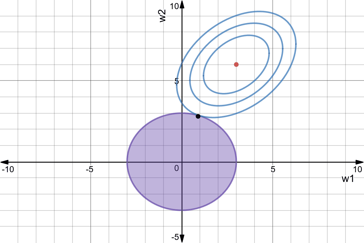
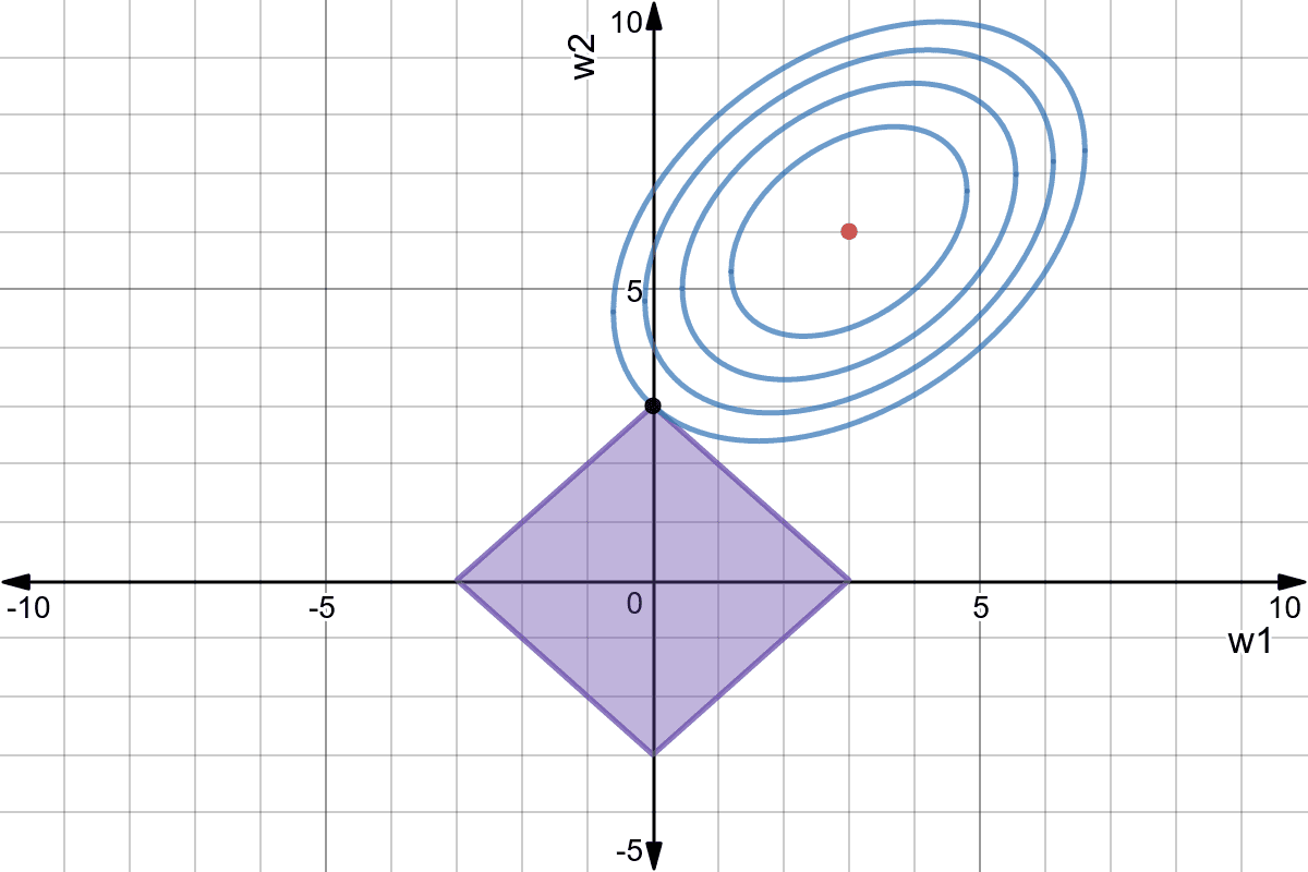
Ridge and Lasso regression
Ridge regression finds the smallest value for the weights that minimize the mse.
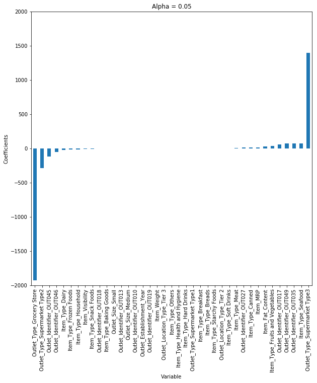
LASSO regression tries to set as many weight to 0 as possible (sparse code).
Both methods depend on the regularization parameter\lambda. Its value determines how important the regularization term should.
Regularization introduce a bias, as the solution found is not the minimum of the mse, but reduces the variance of the estimation, as small weights are less sensible to noise.
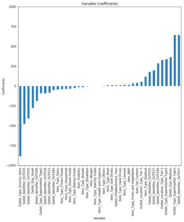
LASSO allows feature selection: features with a zero weight can be removed from the training set.
Linear regression
LASSO
L1+L2 regularization - ElasticNet
An ElasticNet is a linear regression using both L1 and L2 regression:


