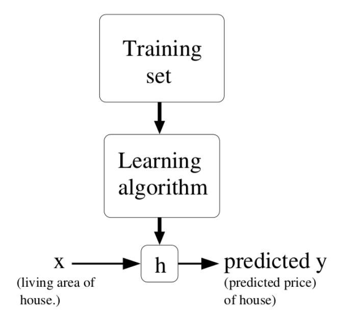
Neurocomputing
Linear classification
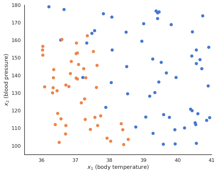
Binary classification
The training data \mathcal{D} is composed of N examples (\mathbf{x}_i, t_i)_{i=1..N} , with a d-dimensional input vector \mathbf{x}_i \in \Re^d and a binary output t_i \in \{-1, +1\}
The data points where t = + 1 are called the positive class, the other the negative class.
Binary classification
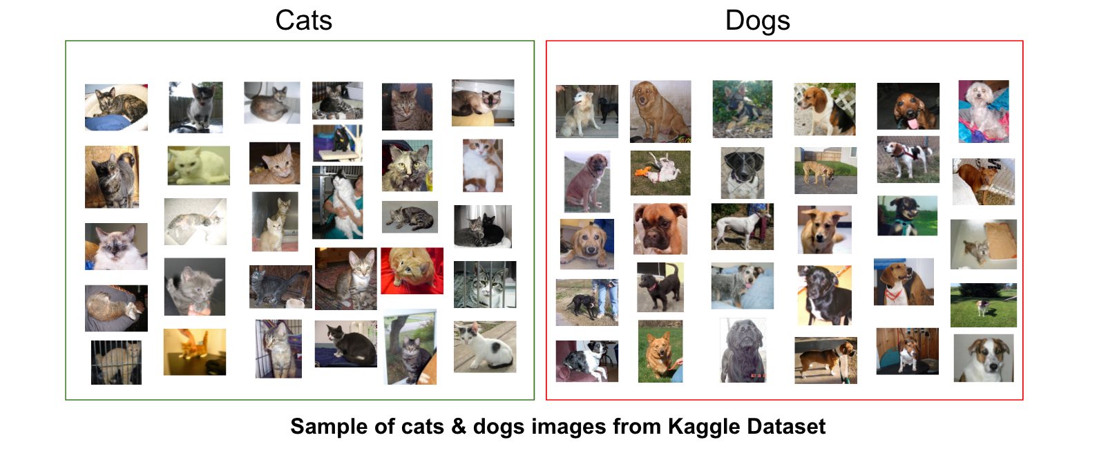
- For example, the inputs \mathbf{x}_i can be images (one dimension per pixel) and the positive class corresponds to cats (t_i = +1), the negative class to dogs (t_i = -1).
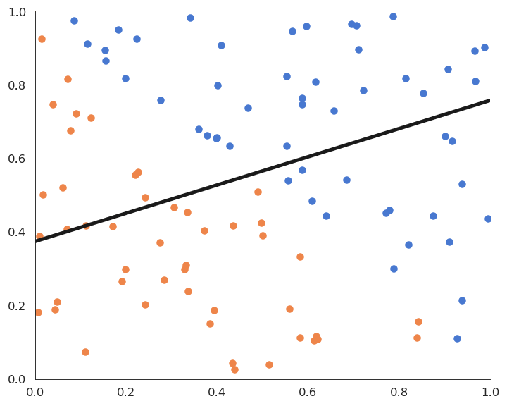
Binary linear classification
- We want to find the hyperplane (\mathbf{w}, b) of \Re^d that correctly separates the two classes.
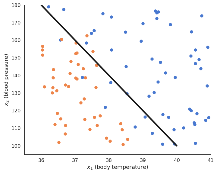
Binary linear classification
For a point \mathbf{x} \in \mathcal{D}, \langle \mathbf{w} \cdot \mathbf{x} \rangle +b is the projection of \mathbf{x} onto the hyperplane (\mathbf{w}, b).
If \langle \mathbf{w} \cdot \mathbf{x} \rangle +b > 0, the point is above the hyperplane.
If \langle \mathbf{w} \cdot \mathbf{x} \rangle +b < 0, the point is below the hyperplane.
If \langle \mathbf{w} \cdot \mathbf{x} \rangle +b = 0, the point is on the hyperplane.
By looking at the sign of \langle \mathbf{w} \cdot \mathbf{x} \rangle +b, we can predict the class of the input:

\text{sign}(\langle \mathbf{w} \cdot \mathbf{x} \rangle +b) = \begin{cases} +1 \; \text{if} \; \langle \mathbf{w} \cdot \mathbf{x} \rangle +b \geq 0 \\ -1 \; \text{if} \; \langle \mathbf{w} \cdot \mathbf{x} \rangle +b < 0 \\ \end{cases}
Binary linear classification
- Binary linear classification can be made by a single artificial neuron using the sign transfer function.
y = f_{\mathbf{w}, b} (\mathbf{x}) = \text{sign} ( \langle \mathbf{w} \cdot \mathbf{x} \rangle +b ) = \text{sign} ( \sum_{j=1}^d w_j \, x_j +b )

- \mathbf{w} is the weight vector and b is the bias.
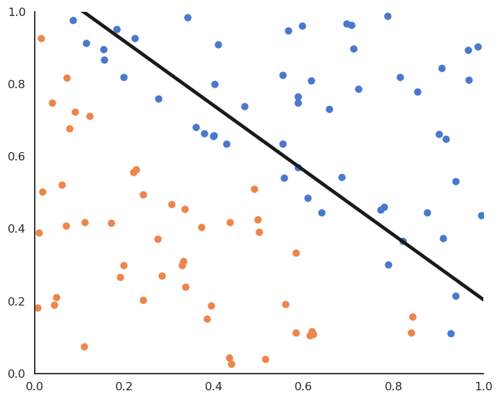
Linearly separable datasets
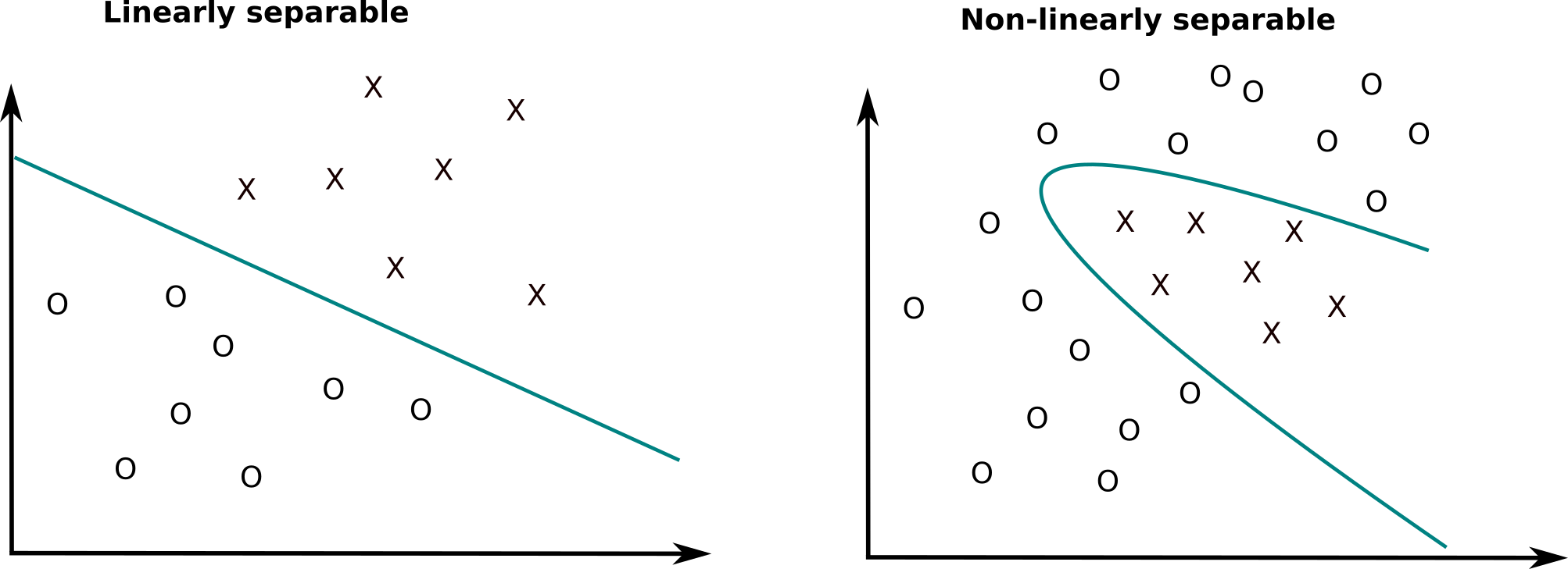
Linear classification is the process of finding an hyperplane (\mathbf{w}, b) that correctly separates the two classes.
If such an hyperplane can be found, the training set is said linearly separable.
Otherwise, the problem is non-linearly separable and other methods have to be applied (MLP, SVM…).
Linear classification as an optimization problem
- Let’s search for the partial derivative of the quadratic error function with respect to the weight vector:
\nabla_\mathbf{w} \, \mathcal{L}(\mathbf{w}, b) = \nabla_\mathbf{w} \, \frac{1}{N} \, \sum_{i=1}^{N} (t_i - y_i )^2 = \frac{1}{N} \, \sum_{i=1}^{N} \nabla_\mathbf{w} \, (t_i - y_i )^2 = \frac{1}{N} \, \sum_{i=1}^{N} \nabla_\mathbf{w} \, \mathcal{l}_i (\mathbf{w}, b)
- Everything is similar to linear regression until we get:
\nabla_\mathbf{w} \, \mathcal{l}_i (\mathbf{w}, b) = - 2 \, (t_i - y_i) \, \nabla_\mathbf{w} \, \text{sign}( \langle \mathbf{w} \cdot \mathbf{x}_i \rangle +b)
- In order to continue with the chain rule, we would need to differentiate \text{sign}(x).
\nabla_\mathbf{w} \, \mathcal{l}_i (\mathbf{w}, b) = - 2 \, (t_i - y_i) \, \text{sign}'( \langle \mathbf{w} \cdot \mathbf{x}_i \rangle +b) \, \mathbf{x}_i
- But the sign function is not differentiable…

Linear classification: batch version
Linear classification: batch version

Linear classification: online version
Linear classification: online version

Stochastic Gradient Descent - SGD
- In practice, we use a trade-off between batch and online learning called Stochastic Gradient Descent (SGD) or Minibatch Gradient Descent.
- The training set is randomly split at each epoch into small chunks of data (a minibatch, usually 32 or 64 examples) and the batch learning rule is applied on each chunk.
\Delta \mathbf{w} = \eta \, \frac{1}{K} \sum_{i=1}^{K} (t_i - y_i) \, \mathbf{x_i}
If the batch size is well chosen, SGD is as stable as batch learning and as fast as online learning.
The minibatches are randomly selected at each epoch (i.i.d).

- Online learning is a stochastic gradient descent with a batch size of 1.
Maximum Likelihood Estimation
Let’s consider N samples \{x_i\}_{i=1}^N independently taken from a normal distribution X.
The probability density function (pdf) of a normal distribution is:
f(x ; \mu, \sigma) = \frac{1}{\sqrt{2\pi \sigma^2}} \, \exp{- \frac{(x - \mu)^2}{2\sigma^2}}
where \mu is the mean of the distribution and \sigma its standard deviation.
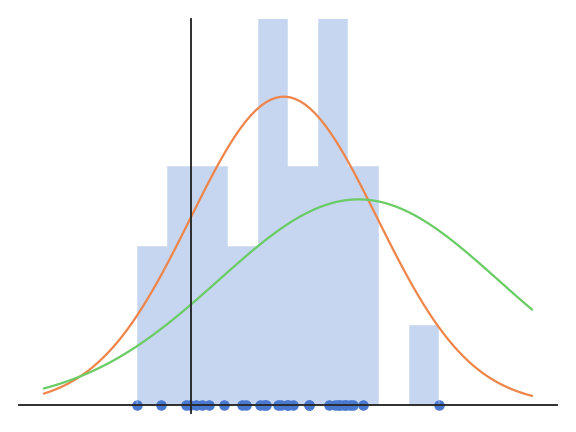
- The problem is to find the values of \mu and \sigma which explain best the observations \{x_i\}_{i=1}^N.
Maximum Likelihood Estimation
- The idea of MLE is to maximize the joint density function for all observations. This function is expressed by the likelihood function:
L(\mu, \sigma) = P( \mathbf{x} ; \mu , \sigma ) = \prod_{i=1}^{N} f(x_i ; \mu, \sigma )
- When the pdf takes high values for all samples, it is quite likely that the samples come from this particular distribution.
The likelihood function reflects how well the parameters \mu and \sigma explain the observations \{x_i\}_{i=1}^N.
Note: the samples must be i.i.d. so that the likelihood is a product.
Reminder: Logistic regression
- We want to perform a regression, but where the targets t_i are bounded betwen 0 and 1.
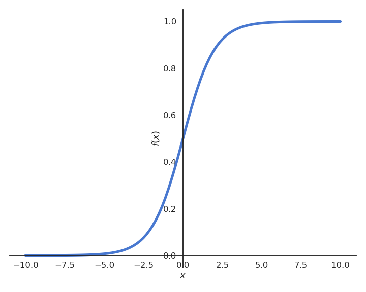
- We can use a logistic function instead of a linear function in order to transform the net activation into an output:
\begin{aligned} y = \sigma(w \, x + b ) = \frac{1}{1+\exp(-w \, x - b )} \end{aligned}
Logistic regression
Logistic regression
\mathbf{w} = 0 \qquad b = 0
for M epochs:
for each sample (\mathbf{x}_i, t_i):
y_i = \sigma( \langle \mathbf{w} \cdot \mathbf{x}_i \rangle + b)
\Delta \mathbf{w} = \eta \, (t_i - y_i) \, \mathbf{x}_i
\Delta b = \eta \, (t_i - y_i)
Logistic regression works just like linear classification, except in the way the prediction is done.
To know to which class \mathbf{x}_i belongs, simply draw a random number between 0 and 1:
if it is smaller than y_i (probability y_i), it belongs to the positive class.
if it is bigger than y_i (probability 1-y_i), it belongs to the negative class.
Alternatively, you can put a hard limit at 0.5:
if y_i > 0.5 then the class is positive.
if y_i < 0.5 then the class is negative.
Logistic regression
Logistic regression and confidence score

Logistic regression also provides a confidence score:
- the closer y is from 0 or 1, the more confident we can be that the classification is correct.
This is particularly important in safety critical applications:
If you detect the positive class but with a confidence of 0.51, you should perhaps not trust the prediction.
If the confidence score is 0.99, you can probably trust the prediction.
Multi-class classification
- Can we perform multi-class classification using the previous methods when t \in \{A, B, C\} instead of t = +1 or -1?

Multi-class classification
- Example of One-vs-All classification: one binary classifier per class.
![]()
Softmax linear classifier

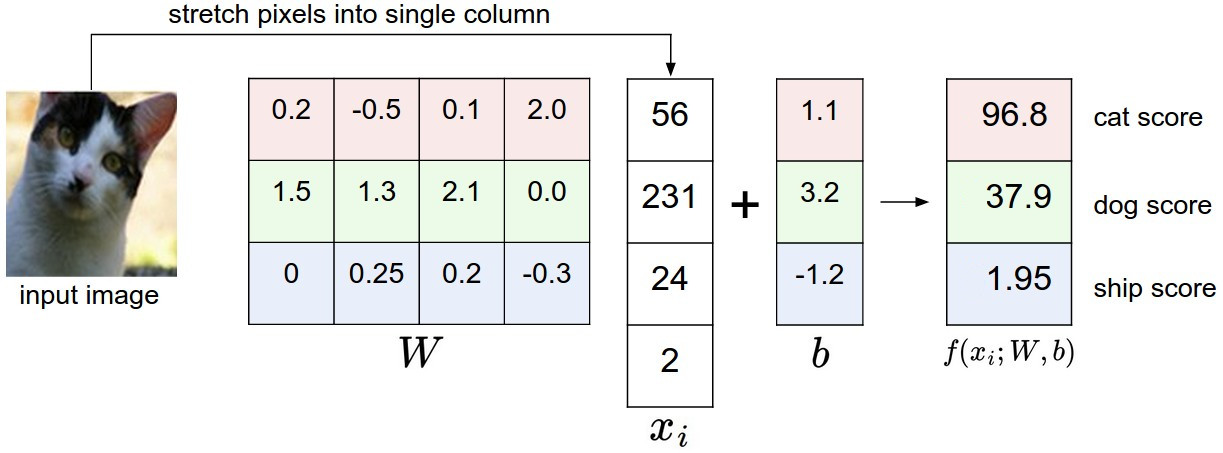
Suppose we have C classes (dog vs. cat vs. ship vs…).
The One-vs-All scheme involves C binary classifiers (\mathbf{w}_i, b_i), each with a weight vector and a bias, working on the same input \mathbf{x}.
y_i = f(\langle \mathbf{w}_i \cdot \mathbf{x} \rangle + b_i)
- Putting all neurons together, we obtain a linear perceptron similar to multiple linear regression:
\mathbf{y} = f(W \times \mathbf{x} + \mathbf{b})
- The C weight vectors form a C \times d weight matrix W, the biases form a vector \mathbf{b}.
Softmax linear classifier
- The net activations form a vector \mathbf{z}:
\mathbf{z} = f_{W, \mathbf{b}}(\mathbf{x}) = W \times \mathbf{x} + \mathbf{b}
Each element z_j of the vector \mathbf{z} is called the logit score of the class:
- the higher the score, the more likely the input belongs to this class.
The logit scores are not probabilities, as they can be negative and do not sum to 1.
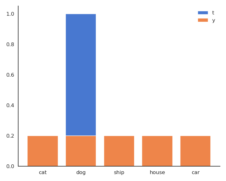
One-hot encoding
How do we represent the ground truth \mathbf{t} for each neuron?
The target vector \mathbf{t} is represented using one-hot encoding.

The binary vector has one element per class: only one element is 1, the others are 0.
Example:
\mathbf{t} = [\text{cat}, \text{dog}, \text{ship}, \text{house}, \text{car}] = [0, 1, 0, 0, 0]
One-hot encoding
The labels can be seen as a probability distribution over the training set, in this case a multinomial distribution (a dice with C sides).
For a given image \mathbf{x} (e.g. a picture of a dog), the conditional pmf is defined by the one-hot encoded vector \mathbf{t}:
P(\mathbf{t} | \mathbf{x}) = [P(\text{cat}| \mathbf{x}), P(\text{dog}| \mathbf{x}), P(\text{ship}| \mathbf{x}), P(\text{house}| \mathbf{x}), P(\text{car}| \mathbf{x})] = [0, 1, 0, 0, 0]
![]()
- We need to transform the logit score \mathbf{z} into a probability distribution P(\mathbf{y} | \mathbf{x}) that should be as close as possible from P(\mathbf{t} | \mathbf{x}).
Softmax linear classifier
- The softmax operator makes sure that the sum of the outputs \mathbf{y} = \{y_i\} over all classes is 1.
y_j = P(\text{class = j} | \mathbf{x}) = \mathcal{S}(z_j) = \frac{\exp(z_j)}{\sum_k \exp(z_k)}
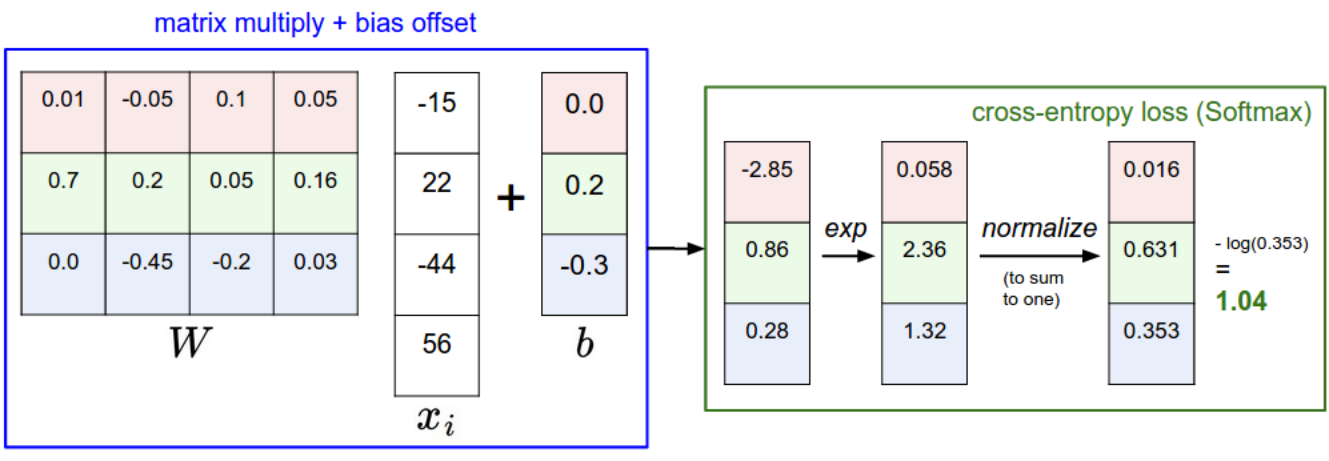
The higher z_j, the higher the probability that the example belongs to class j.
This is very similar to logistic regression for soft classification, except that we have multiple classes.
Cross-entropy loss function
- We cannot use the mse as a loss function, as the softmax function would be hard to differentiate:
\text{mse}(W, \mathbf{b}) = \sum_j (t_{j} - \frac{\exp(z_j)}{\sum_k \exp(z_k)})^2
![]()
We actually want to minimize the statistical distance netween two distributions:
The model outputs a multinomial probability distribution \mathbf{y} for an input \mathbf{x}: P(\mathbf{y} | \mathbf{x}; W, \mathbf{b}).
The one-hot encoded classes also come from a multinomial probability distribution P(\mathbf{t} | \mathbf{x}).
We search which parameters (W, \mathbf{b}) make the two distributions P(\mathbf{y} | \mathbf{x}; W, \mathbf{b}) and P(\mathbf{t} | \mathbf{x}) close.
Cross-entropy loss function
The training data \{\mathbf{x}_i, \mathbf{t}_i\} represents samples from P(\mathbf{t} | \mathbf{x}).
P(\mathbf{y} | \mathbf{x}; W, \mathbf{b}) is a good model of the data when the two distributions are close, i.e. when the negative log-likelihood of each sample under the model is small.

- For an input \mathbf{x}, we minimize the cross-entropy between the target distribution and the predicted outputs:
\mathcal{l}(W, \mathbf{b}) = \mathcal{H}(\mathbf{t} | \mathbf{x}, \mathbf{y} | \mathbf{x}) = \mathbb{E}_{t \sim P(\mathbf{t} | \mathbf{x})} [ - \log P(\mathbf{y} = t | \mathbf{x})]
Cross-entropy and negative log-likelihood
![]()
- The cross-entropy samples from \mathbf{t} | \mathbf{x}:
\mathcal{l}(W, \mathbf{b}) = \mathcal{H}(\mathbf{t} | \mathbf{x}, \mathbf{y} | \mathbf{x}) = \mathbb{E}_{t \sim P(\mathbf{t} | \mathbf{x})} [ - \log P(\mathbf{y} = t | \mathbf{x})] = - \sum_{j=1}^C P(t_j | \mathbf{x}) \, \log P(y_j = t_j | \mathbf{x})
- For a given input \mathbf{x}, \mathbf{t} is non-zero only for the correct class t^*, as \mathbf{t} is a one-hot encoded vector [0, 1, 0, 0, 0]:
\mathcal{l}(W, \mathbf{b}) = - \log P(\mathbf{y} = t^* | \mathbf{x})
- If we note j^* the index of the correct class t^*, the cross entropy is simply:
\mathcal{l}(W, \mathbf{b}) = - \log y_{j^*}
Cross-entropy and negative log-likelihood

- As only one element of \mathbf{t} is non-zero, the cross-entropy is the same as the negative log-likelihood of the prediction for the true label:
\mathcal{l}(W, \mathbf{b}) = - \log y_{j^*}
The minimum of - \log y is obtained when y =1:
- We want to classifier to output a probability 1 for the true label.
Because of the softmax activation function, the probability for the other classes should become closer from 0.
y_j = P(\text{class = j}) = \frac{\exp(z_j)}{\sum_k \exp(z_k)}
- Minimizing the cross-entropy / negative log-likelihood pushes the output distribution \mathbf{y} | \mathbf{x} to be as close as possible to the target distribution \mathbf{t} | \mathbf{x}.
Cross-entropy loss function
Cross-entropy loss function
- As \mathbf{t} is a binary vector [0, 1, 0, 0, 0], the cross-entropy / negative log-likelihood can also be noted as the dot product between \mathbf{t} and \log \mathbf{y}:
\mathcal{l}(W, \mathbf{b}) = - \langle \mathbf{t} \cdot \log \mathbf{y} \rangle = - \sum_{j=1}^C t_j \, \log y_j = - \log y_{j^*}

- The cross-entropy loss function is then the expectation over the training set of the individual cross-entropies: \mathcal{L}(W, \mathbf{b}) = \mathbb{E}_{\mathbf{x}, \mathbf{t} \sim \mathcal{D}} [- \langle \mathbf{t} \cdot \log \mathbf{y} \rangle ] \approx \frac{1}{N} \sum_{i=1}^N - \langle \mathbf{t}_i \cdot \log \mathbf{y}_i \rangle
Softmax linear classifier
- We first compute the logit scores \mathbf{z} using a linear layer:
\mathbf{z} = W \times \mathbf{x} + \mathbf{b}
- We turn them into probabilities \mathbf{y} using the softmax activation function:
y_j = \frac{\exp(z_j)}{\sum_k \exp(z_k)}
- We minimize the cross-entropy / negative log-likelihood on the training set:
\mathcal{L}(W, \mathbf{b}) = \mathbb{E}_{\mathbf{x}, \mathbf{t} \sim \mathcal{D}} [ - \langle \mathbf{t} \cdot \log \mathbf{y} \rangle]
which simplifies into the delta learning rule:
\begin{cases} \Delta W = \eta \, (\mathbf{t} - \mathbf{y} ) \times \mathbf{x}^T \\ \\ \Delta \mathbf{b} = \eta \, (\mathbf{t} - \mathbf{y} ) \\ \end{cases}
Comparison of linear classification and regression
- Classification and regression differ in the nature of their outputs: in classification they are discrete, in regression they are continuous values.
- However, when trying to minimize the mismatch between a model \mathbf{y} and the real data \mathbf{t}, we have found the same delta learning rule:
\begin{cases} \Delta W = \eta \, (\mathbf{t} - \mathbf{y} ) \times \mathbf{x}^T \\ \\ \Delta \mathbf{b} = \eta \, (\mathbf{t} - \mathbf{y} ) \\ \end{cases}
- Regression and classification are in the end the same problem for us. The only things that needs to be adapted is the activation function of the output and the loss function.
- For regression, we use linear activation functions and the mean square error (mse):
\mathcal{L}(W, \mathbf{b}) = \mathbb{E}_{\mathbf{x}, \mathbf{t} \sim \mathcal{D}} [ ||\mathbf{t} - \mathbf{y}||^2 ]
- For classification, we use the softmax activation function and the cross-entropy (negative log-likelihood) loss function.
\mathcal{L}(W, \mathbf{b}) = \mathbb{E}_{\mathbf{x}, \mathbf{t} \sim \mathcal{D}} [ - \langle \mathbf{t} \cdot \log \mathbf{y} \rangle]
Multi-label classification
- For multi-label classification, we can simply use the logistic activation function for the output neurons:
\mathbf{y} = \sigma(W \times \mathbf{x} + \mathbf{b})
- The outputs are between 0 and 1, but they do not sum to one. Each output neuron performs logistic regression for soft classification on their class:
y_j = P(\text{class} = j | \mathbf{x})
- Each output neuron y_j has a binary target t_j (one-vs-the-rest) and has to minimize the negative log-likelihood:
\mathcal{l}_j(W, \mathbf{b}) = - t_j \, \log y_j + (1 - t_j) \, \log( 1- y_j)
- The binary cross-entropy loss is the sum of the negative log-likelihood for each class: \mathcal{L}(W, \mathbf{b}) = \mathbb{E}_{\mathcal{D}} [- \sum_{j=1}^C t_j \, \log y_j + (1 - t_j) \, \log( 1- y_j)]
Training vs. Generalization error
The training error is the error made on the training set.
- Easy to measure for classification: number of misclassified examples divided by the total number.
\epsilon_\mathcal{D} = \dfrac{\text{number of misclassifications}}{\text{number of examples}}
- Totally irrelevant on usage: reading the training set has a training error of 0%.
What matters is the generalization error, which is the error that will be made on new examples (not used during learning).
Much harder to measure (potentially infinite number of new examples, what is the correct answer?).
Often approximated by the empirical error on the test set: one keeps a number of training examples out of the learning phase and one tests the performance on them.
Need for cross-validation to detect overfitting.
Overfitting in regression
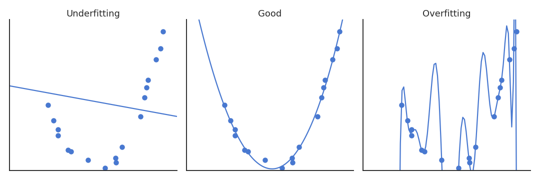
Overfitting in classification

Classification errors
Confusion matrix
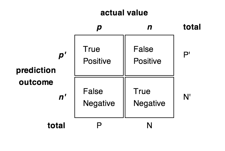
Classification errors can also depend on the class:
False Positive errors (FP, false alarm, type I) is when the classifier predicts a positive class for a negative example.
False Negative errors (FN, miss, type II) is when the classifier predicts a negative class for a positive example.
True Positive (TP) and True Negative (TN) are correctly classified examples.
Is it better to fail to detect a cancer (FN) or to incorrectly predict one (FP)?
Classification errors

- Error
\epsilon = \frac{\text{FP} + \text{FN}}{\text{TP} + \text{FP} + \text{TN} + \text{FN}}
- Accuracy (1 - error)
\text{acc} = \frac{\text{TP} + \text{TN}}{\text{TP} + \text{FP} + \text{TN} + \text{FN}}
- Recall (hit rate, sensitivity) and Precision (specificity)
R = \frac{\text{TP}}{\text{TP} + \text{FN}} \;\; P = \frac{\text{TP}}{\text{TP} + \text{FP}}
- F1 score = harmonic mean of precision and recall
\text{F1} = \frac{2\, P \, R}{P + R}
Confusion matrix
For multiclass classification problems, the confusion matrix tells how many examples are correctly classified and where confusion happens.
One axis is the predicted class, the other is the target class.
Each element of the matrix tells how many examples are classified or misclassified.
The matrix should be as diagonal as possible.
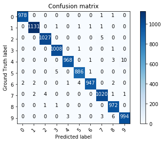
- Using
scikit-learn:
from sklearn.metrics import confusion_matrix

m = confusion_matrix(t, y)