Neurocomputing
Learning theory
Julien Vitay
Professur für Künstliche Intelligenz - Fakultät für Informatik
Non-linear regression and classification
We have seen sofar linear learning algorithms for regression and classification.
Most interesting problems are non-linear: classes are not linearly separable, the output is not a linear function of the input, etc…
Do we need totally new methods, or can we re-use our linear algorithms?
Vapnik-Chervonenkis dimension of an hypothesis class
How many data examples can be correctly classified by a linear model in \Re^d?
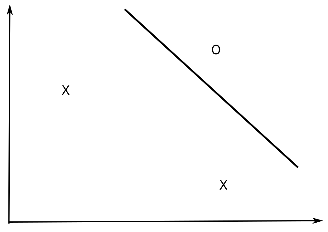
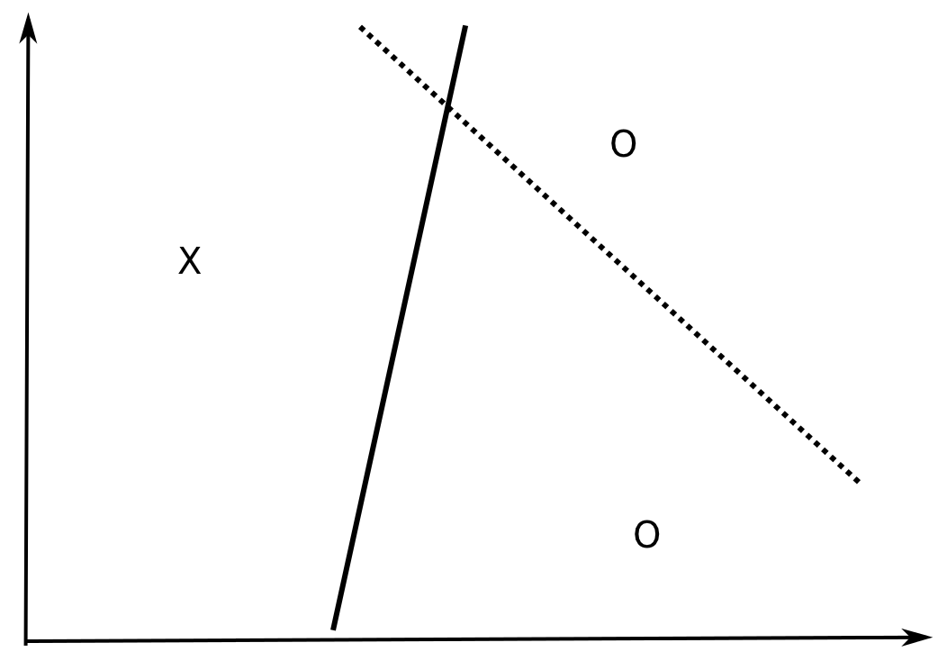
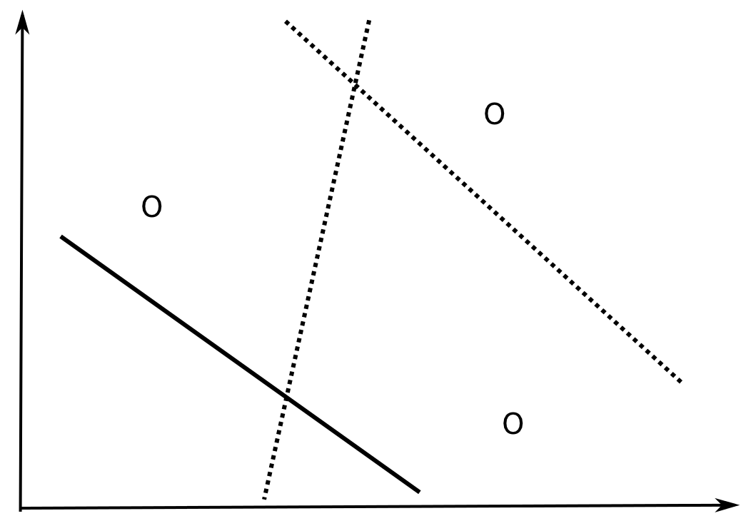
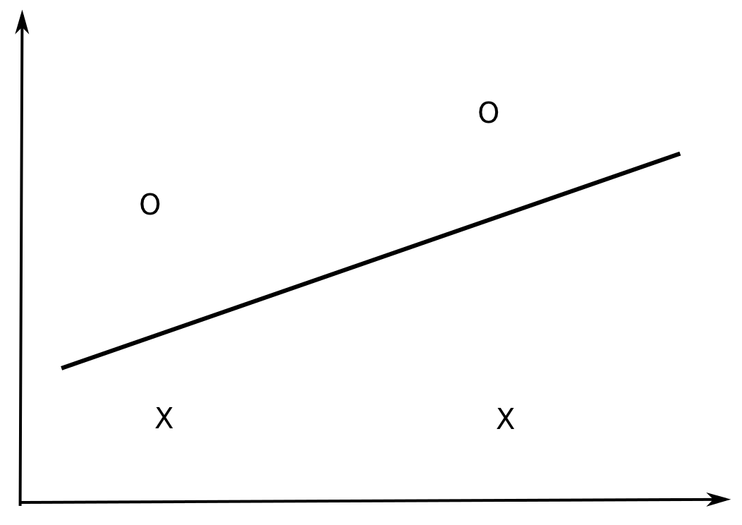
In \Re^2, all dichotomies of three non-aligned examples can be correctly classified by a linear model (y = w_o + w_1 \cdot x_1 + w_2 \cdot x_2).
Vapnik-Chervonenkis dimension of an hypothesis class
How many data examples can be correctly classified by a linear model in \Re^d?
In \Re^2, all dichotomies of three non-aligned examples can be correctly classified by a linear model (y = w_o + w_1 \cdot x_1 + w_2 \cdot x_2).
Vapnik-Chervonenkis dimension of an hypothesis class
How many data examples can be correctly classified by a linear model in \Re^d?
In \Re^2, all dichotomies of three non-aligned examples can be correctly classified by a linear model (y = w_o + w_1 \cdot x_1 + w_2 \cdot x_2).
Vapnik-Chervonenkis dimension of an hypothesis class
How many data examples can be correctly classified by a linear model in \Re^d?
In \Re^2, all dichotomies of three non-aligned examples can be correctly classified by a linear model (y = w_o + w_1 \cdot x_1 + w_2 \cdot x_2).
Vapnik-Chervonenkis dimension of an hypothesis class
How many data examples can be correctly classified by a linear model in \Re^d?
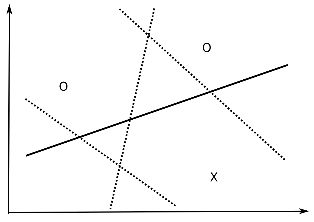
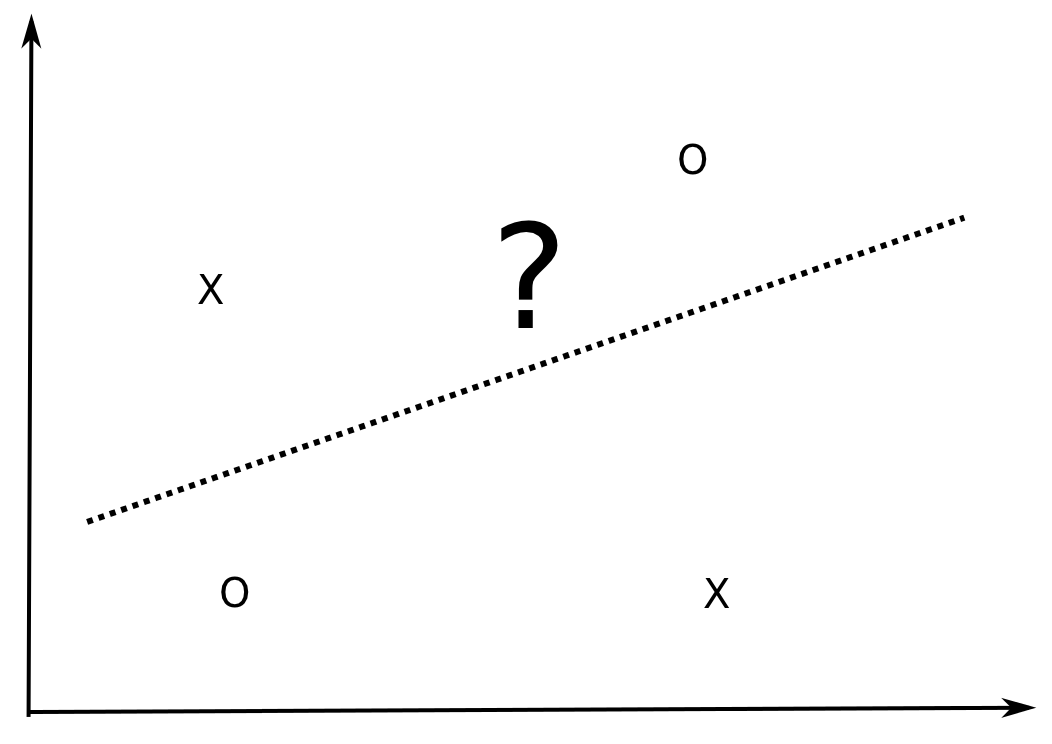
However, there exists sets of four examples in \Re^2 which can NOT be correctly classified by a linear model, i.e. they are not linearly separable.
Vapnik-Chervonenkis dimension of an hypothesis class
How many data examples can be correctly classified by a linear model in \Re^d?
However, there exists sets of four examples in \Re^2 which can NOT be correctly classified by a linear model, i.e. they are not linearly separable.
Non-linearly separable data
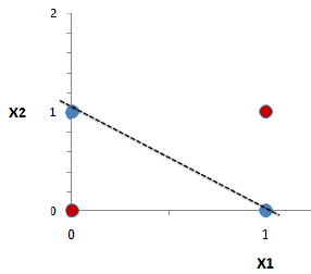
- The XOR function in \Re^2 is for example not linearly separable, i.e. the Perceptron algorithm can not converge.
The probability that a set of 3 (non-aligned) points in \Re^2 is linearly separable is 1, but the probability that a set of four points is linearly separable is smaller than 1 (but not zero).
When a class of hypotheses \mathcal{H} can correctly classify all points of a training set \mathcal{D}, we say that \mathcal{H} shatters \mathcal{D}.
Vapnik-Chervonenkis dimension of an hypothesis class
The Vapnik-Chervonenkis dimension \text{VC}_\text{dim} (\mathcal{H}) of an hypothesis class \mathcal{H} is defined as the maximal number of training examples that \mathcal{H} can shatter.
We saw that in \Re^2, this dimension is 3:
\text{VC}_\text{dim} (\text{Linear}(\Re^2) ) = 3
- This can be generalized to linear classifiers in \Re^d:
\text{VC}_\text{dim} (\text{Linear}(\Re^d) ) = d+1
This corresponds to the number of free parameters of the linear classifier:
- d parameters for the weight vector, 1 for the bias.
Given any set of (d+1) examples in \Re^d, there exists a linear classifier able to classify them perfectly.
For other types of (non-linear) hypotheses, the VC dimension is generally proportional to the number of free parameters.
But regularization reduces the VC dimension of the classifier.
Vapnik-Chervonenkis theorem
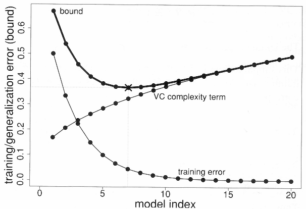
- The generalization error \epsilon(h) of an hypothesis h taken from a class \mathcal{H} of finite VC dimension and trained on N samples of \mathcal{S} is bounded by the sum of the training error \hat{\epsilon}_{\mathcal{S}}(h) and the VC complexity term:
\epsilon(h) \leq \hat{\epsilon}_{\mathcal{S}}(h) + \sqrt{\frac{\text{VC}_\text{dim} (\mathcal{H}) \cdot (1 + \log(\frac{2\cdot N}{\text{VC}_\text{dim} (\mathcal{H})})) - \log(\frac{\delta}{4})}{N}}
with probability 1-\delta, if \text{VC}_\text{dim} (\mathcal{H}) << N.
Structural risk minimization
\epsilon(h) \leq \hat{\epsilon}_{\mathcal{S}(h)} + \sqrt{\frac{\text{VC}_\text{dim} (\mathcal{H}) \cdot (1 + \log(\frac{2\cdot N}{\text{VC}_\text{dim} (\mathcal{H})})) - \log(\frac{\delta}{4})}{N}}
Structural risk minimization
\epsilon(h) \leq \hat{\epsilon}_{\mathcal{S}(h)} + \sqrt{\frac{\text{VC}_\text{dim} (\mathcal{H}) \cdot (1 + \log(\frac{2\cdot N}{\text{VC}_\text{dim} (\mathcal{H})})) - \log(\frac{\delta}{4})}{N}}
The generalization error increases with the VC dimension, while the training error decreases.
Structural risk minimization is an alternative method to cross-validation.
The VC dimensions of various classes of hypothesis are already known (~ number of free parameters).
This bounds tells how many training samples are needed by a given hypothesis class in order to obtain a satisfying generalization error.
- The more complex the model, the more training data you will need to get a good generalization error!
\epsilon(h) \approx \frac{\text{VC}_\text{dim} (\mathcal{H})}{N}
A learning algorithm should only try to minimize the training error, as the VC complexity term only depends on the model.
This term is only an upper bound: most of the time, the real bound is usually 100 times smaller.
Implication for non-linear classifiers
- The VC dimension of linear classifiers in \Re^d is:
\text{VC}_\text{dim} (\text{Linear}(\Re^d) ) = d+1
Given any set of (d+1) examples in \Re^d, there exists a linear classifier able to classify them perfectly.
For N >> d the probability of having training errors becomes huge (the data is generally not linearly separable).
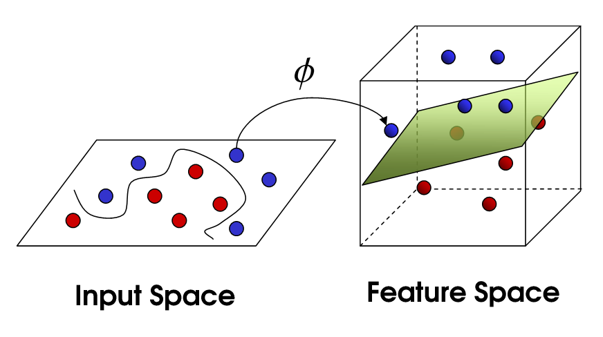
- If we project the input data onto a space with sufficiently high dimensions, it becomes then possible to find a linear classifier on this projection space that is able to classify the data!
However, if the space has too many dimensions, the VC dimension will increase and the generalization error will increase.
Basic principle of all non-linear methods: multi-layer perceptron, radial-basis-function networks, support-vector machines…
Cover’s theorem on the separability of patterns (1965)
A complex pattern-classification problem, cast in a high dimensional space non-linearly, is more likely to be linearly separable than in a low-dimensional space, provided that the space is not densely populated.
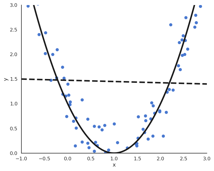
Polynomial features
- For the polynomial regression of order p:
y = f_{\mathbf{w}, b}(x) = w_1 \, x + w_2 \, x^2 + \ldots + w_p \, x^p + b
the vector \mathbf{x} = \begin{bmatrix} x \\ x^2 \\ \ldots \\ x^p \end{bmatrix} defines a feature space for the input x.
The elements of the feature space are called polynomial features.
We can define polynomial features of more than one variable, e.g. x^2 \, y, x^3 \, y^4, etc.
We then apply multiple linear regression (MLR) on the polynomial feature space to find the parameters:
\Delta \mathbf{w} = \eta \, (t - y) \, \mathbf{x}
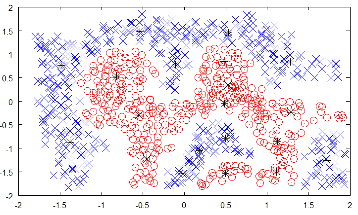
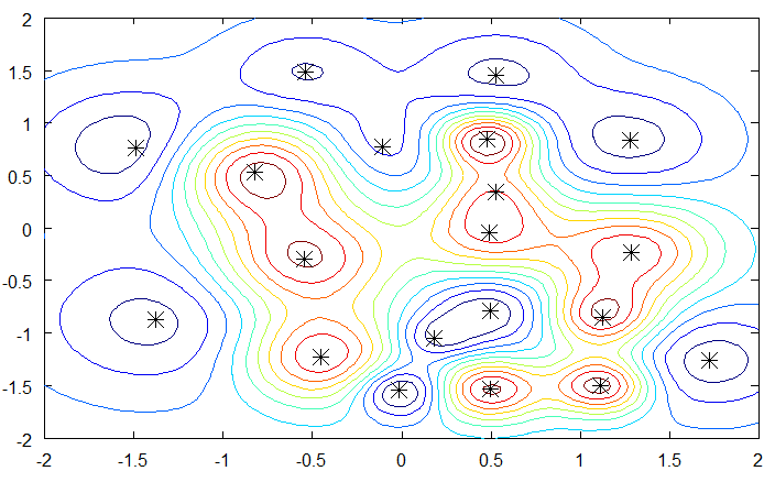
Radial-basis function networks
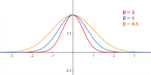
- Radial-basis function (RBF) networks samples a subset of K training examples and form the feature space using a gaussian kernel:
\phi(\mathbf{x}) = \begin{bmatrix} \varphi(\mathbf{x} - \mathbf{x}_1) \\ \varphi(\mathbf{x} - \mathbf{x}_2) \\ \ldots \\ \varphi(\mathbf{x} - \mathbf{x}_K) \end{bmatrix}
with \varphi(\mathbf{x} - \mathbf{x}_i) = \exp - \beta \, ||\mathbf{x} - \mathbf{x}_i||^2 decreasing with the distance between the vectors.
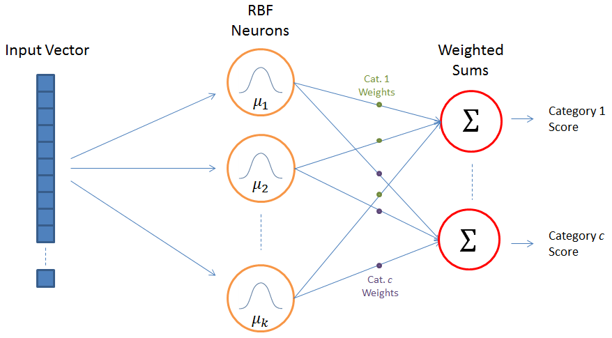
Radial-basis function networks
- By applying a linear classification algorithm on the RBF feature space:
\mathbf{y} = f(W \times \phi(\mathbf{x}) + \mathbf{b})
we obtain a smooth non-linear partition of the input space.
- The width of the gaussian kernel allows distance-based generalization.
3 - Kernel algorithms (optional)
Kernel perceptron
What happens during online Perceptron learning?
If an example \mathbf{x}_i is correctly classified (y_i = t_i), the weight vector does not change.
\mathbf{w} \leftarrow \mathbf{w}
- If an example \mathbf{x}_i is miscorrectly classified (y_i \neq t_i), the weight vector is increased from t_i \, \mathbf{x}_i.
\mathbf{w} \leftarrow \mathbf{w} + 2 \, \eta \, t_i \, \mathbf{x}_i
Primal form of the online Perceptron algorithm
- If you initialize the weight vector to 0, its final value will therefore be a linear combination of the input samples:
\mathbf{w} = \sum_{i=1}^N \alpha_i \, t_i \, \mathbf{x}_i
- The coefficients \alpha_i represent the embedding strength of each example, i.e. how often they were misclassified.
Kernel perceptron
- With \mathbf{w} = \sum_{i=1}^N \alpha_i \, t_i \, \mathbf{x}_i, the prediction for an input \mathbf{x} only depends on the training samples and their \alpha_i value:
y = \text{sign}( \sum_{i=1}^N \alpha_i \, t_i \, \langle \mathbf{x}_i \cdot \mathbf{x} \rangle)
To make a prediction y, we need the dot product between the input \mathbf{x} and all training examples \mathbf{x}_i.
We ignore the bias here, but it can be added back.
Dual form of the online Perceptron algorithm
This dual form of the Perceptron algorithm is strictly equivalent to its primal form.
It needs one parameter \alpha_i per training example instead of a weight vector (N >> d), but relies on dot products between vectors.
Kernel perceptron
- Why is it interesting to have an algorithm relying on dot products?
y = \text{sign}( \sum_{i=1}^N \alpha_i \, t_i \, \langle \mathbf{x}_i \cdot \mathbf{x} \rangle)
- You can project the inputs \mathbf{x} to a feature space \phi(\mathbf{x}) and apply the same algorithm:
y = \text{sign}( \sum_{i=1}^N \alpha_i \, t_i \, \langle \phi(\mathbf{x}_i) \cdot \phi(\mathbf{x}) \rangle)
- But you do not need to compute the dot product in the feature space, all you need to know is its result.
K(\mathbf{x}_i, \mathbf{x}) = \langle \phi(\mathbf{x}_i) \cdot \phi(\mathbf{x}) \rangle
- Kernel trick: A kernel K(\mathbf{x}, \mathbf{z}) allows to compute the dot product between the feature space representation of two vectors without ever computing these representations!
Example of the polynomial kernel
- Let’s consider the quadratic kernel in \Re^3:
\begin{aligned}
\forall (\mathbf{x}, \mathbf{z}) \in \Re^3 \times \Re^3 & \\
& \\
K(\mathbf{x}, \mathbf{z}) &= ( \langle \mathbf{x} \cdot \mathbf{z} \rangle)^2 \\
&= (\sum_{i=1}^3 x_i \cdot z_i) \cdot (\sum_{j=1}^3 x_j \cdot z_j) \\
&= \sum_{i=1}^3 \sum_{j=1}^3 (x_i \cdot x_j) \cdot ( z_i \cdot z_j) \\
&= \langle \phi(\mathbf{x}) \cdot \phi(\mathbf{z}) \rangle \\
\end{aligned}
\text{with:} \qquad \phi(\mathbf{x}) = \begin{bmatrix}
x_1 \cdot x_1 \\
x_1 \cdot x_2 \\
x_1 \cdot x_3 \\
x_2 \cdot x_1 \\
x_2 \cdot x_2 \\
x_2 \cdot x_3 \\
x_3 \cdot x_1 \\
x_3 \cdot x_2 \\
x_3 \cdot x_3 \end{bmatrix}
- The quadratic kernel implicitely transforms an input space with three dimensions into a feature space of 9 dimensions.
Example of the polynomial kernel
- More generally, the polynomial kernel in \Re^d of degree p:
\begin{align*}
\forall (\mathbf{x}, \mathbf{z}) \in \Re^d \times \Re^d \qquad K(\mathbf{x}, \mathbf{z}) &= ( \langle \mathbf{x} \cdot \mathbf{z} \rangle)^p \\
&= \langle \phi(\mathbf{x}) \cdot \phi(\mathbf{z}) \rangle
\end{align*}
transforms the input from a space with d dimensions into a feature space of d^p dimensions.
While the inner product in the feature space would require O(d^p) operations, the calculation of the kernel directly in the input space only requires O(d) operations.
This is called the kernel trick: when a linear algorithm only relies on the dot product between input vectors, it can be safely projected into a higher dimensional feature space through a kernel function, without increasing too much its computational complexity, and without ever computing the values in the feature space.
Kernel perceptron
- The kernel perceptron is the dual form of the Perceptron algorithm using a kernel.
- Depending on the kernel, the implicit dimensionality of the feature space can even be infinite!
- Linear kernel: d dimensions.
K(\mathbf{x},\mathbf{z}) = \langle \mathbf{x} \cdot \mathbf{z} \rangle
- Polynomial kernel: d^p dimensions.
K(\mathbf{x},\mathbf{z}) = (\langle \mathbf{x} \cdot \mathbf{z} \rangle)^p
- Gaussian kernel (or RBF kernel): \infty dimensions.
K(\mathbf{x},\mathbf{z}) = \exp(-\frac{\| \mathbf{x} - \mathbf{z} \|^2}{2\sigma^2})
- Hyperbolic tangent kernel: \infty dimensions.
k(\mathbf{x},\mathbf{z})=\tanh(\langle \kappa \mathbf{x} \cdot \mathbf{z} \rangle +c)
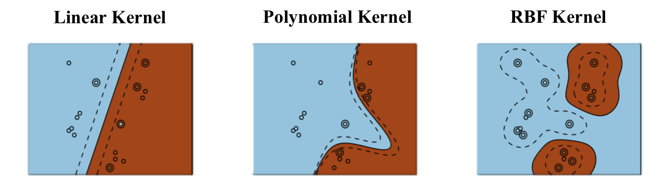
Examples of kernels
In practice, the choice of the kernel family depends more on the nature of data (text, image…) and its distribution than on the complexity of the learning problem.
RBF kernels tend to “group” positive examples together.
Polynomial kernels are more like “distorted” hyperplanes.
Kernels have parameters (p, \sigma…) which have to found using cross-validation.
Support vector machines
Support vector machines (SVM) extend the idea of a kernel perceptron using a different linear learning algorithm, the maximum margin classifier.
Using Lagrange optimization and regularization, the maximal margin classifer tries to maximize the “safety zone” (geometric margin) between the classifier and the training examples.
It also tries to reduce the number of non-zero \alpha_i coefficients to keep the complexity of the classifier bounded, thereby improving the generalization:
\mathbf{y} = \text{sign}(\sum_{i=1}^{N_{SV}} \alpha_i \, t_i \, K(\mathbf{x}_i, \mathbf{x}) + b)
Coupled with a good kernel, a SVM can efficiently solve non-linear classification problems without overfitting.
SVMs were the weapon of choice before the deep learning era, which deals better with huge datasets.