Neurocomputing

Multi-layer Perceptron

Julien Vitay

Professur für Künstliche Intelligenz - Fakultät für Informatik

1 - Multi-layer perceptron

Multi-layer perceptron

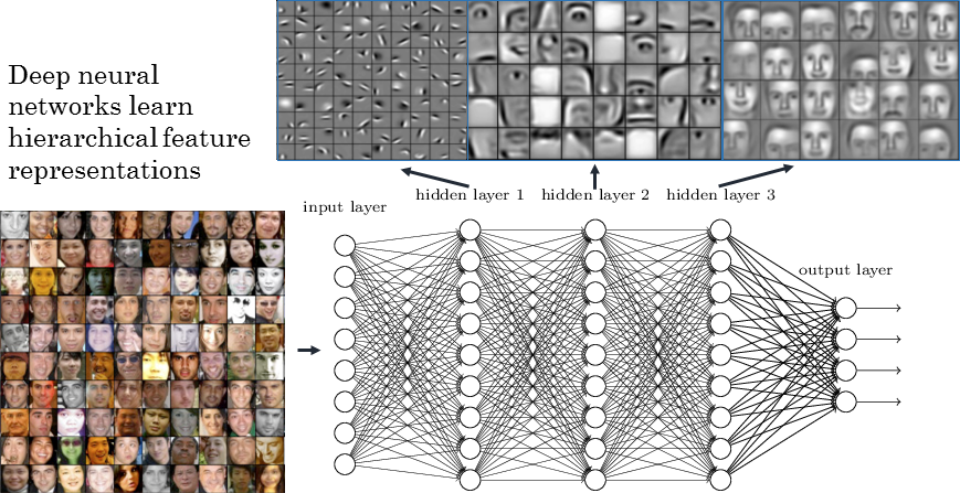
• A Multi-Layer Perceptron (MLP) or feedforward neural network is composed of:

  • an input layer for the input vector \mathbf{x}

  • one or several hidden layers allowing to project non-linearly the input into a space of higher dimensions \mathbf{h}_1, \mathbf{h}_2, \mathbf{h}_3, \ldots.

  • an output layer for the output \mathbf{y}.

• If there is a single hidden layer \mathbf{h}, it corresponds to the feature space.

• Each layer takes inputs from the previous layer.

• If the hidden layer is adequately chosen, the output neurons can learn to replicate the desired output \mathbf{t}.

Fully-connected layer

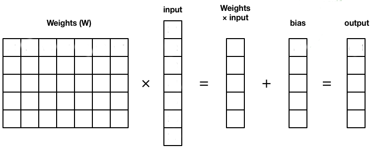
• The operation performed by each layer can be written in the form of a matrix-vector multiplication:

\mathbf{h} = f(\textbf{net}_\mathbf{h}) = f(W^1 \, \mathbf{x} + \mathbf{b}^1) \mathbf{y} = f(\textbf{net}_\mathbf{y}) = f(W^2 \, \mathbf{h} + \mathbf{b}^2)

• Fully-connected layers (FC) transform an input vector \mathbf{x} into a new vector \mathbf{h} by multiplying it by a weight matrix W and adding a bias vector \mathbf{b}.

• A non-linear activation function transforms each element of the net activation.

Activation functions

Modern activation functions

• Rectified linear function - ReLU (output is continuous and positive).

f(x) = \max(0, x) = \begin{cases} x \quad \text{if} \quad x \geq 0 \\ 0 \quad \text{otherwise.} \end{cases}

• Parametric Rectifier Linear Unit - PReLU (output is continuous).

f(x) = \begin{cases} x \quad \text{if} \quad x \geq 0 \\ \alpha \, x \quad \text{otherwise.}\end{cases}

Softmax activation function

Source http://cs231n.github.io/linear-classify

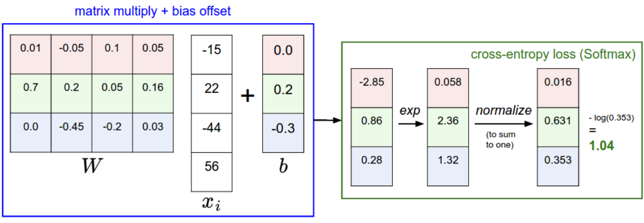
• For classification problems, the softmax activation function can be used in the output layer to make sure that the sum of the outputs \mathbf{y} = \{y_j\} over all output neurons is one.

y_j = P(\text{class = j}) = \frac{\exp(\text{net}_j)}{\sum_k \exp(\text{net}_k)}

• The higher the net activation \text{net}_j, the higher the probability that the example belongs to class j.

• Softmax is not per se a transfer function (not local to each neuron), but the idea is similar.

Why non-linear activation functions?

• Why not use the linear function f(x) = x in the hidden layer?

\mathbf{h} = W^1 \, \mathbf{x} + \mathbf{b}^1 \mathbf{y} = W^2 \, \mathbf{h} + \mathbf{b}^2

• The equivalent function would be linear…

\begin{align*} \mathbf{y} &= W^2 \, (W^1 \, \mathbf{x} + \mathbf{b}^1) + \mathbf{b}^2 \\ &= (W^2 \, W^1) \, \mathbf{x} + (W^2 \, \mathbf{b}^1 + \mathbf{b}^2) \\ &= W \, \mathbf{x} + \mathbf{b} \\ \end{align*}

• Remember Cover’s theorem:

A complex pattern-classification problem, cast in a high dimensional space non-linearly, is more likely to be linearly separable than in a low-dimensional space, provided that the space is not densely populated.

• In practice it does not matter how non-linear the function is (e.g PReLU is almost linear), but there must be at least one non-linearity.

Training a MLP : loss functions

• We have a training set composed of N input/output pairs (\mathbf{x}_i, \mathbf{t}_i)_{i=1..N}.

Optimization problem

What are the free parameters \theta (weights W^1, W^2 and biases \textbf{b}^1, \textbf{b}^2) making the prediction \mathbf{y} as close as possible from the desired output \mathbf{t}?

• We define a loss function \mathcal{L}(\theta) of the free parameters which should be minimized:

  • For regression problems, we take the mean square error (mse):

  \mathcal{L}_\text{reg}(\theta) = \mathbb{E}_{\mathbf{x}, \mathbf{t} \in \mathcal{D}} [ ||\mathbf{t} - \mathbf{y}||^2 ]

  • For classification problems, we take the cross-entropy or negative log-likelihood on a softmax output layer:

  \mathcal{L}_\text{class}(\theta) = \mathbb{E}_{\mathbf{x}, \mathbf{t} \sim \mathcal{D}} [ - \langle \mathbf{t} \cdot \log \mathbf{y} \rangle]

Training a MLP : optimizer

• To minimize the chosen loss function, we are going to use stochastic gradient descent iteratively until the network converges:

\begin{cases} \Delta W^1 = - \eta \, \nabla_{W^1} \, \mathcal{L}(\theta) \\ \\ \Delta \mathbf{b}^1 = - \eta \, \nabla_{\mathbf{b}^1} \, \mathcal{L}(\theta) \\ \\ \Delta W^2 = - \eta \, \nabla_{W^2} \, \mathcal{L}(\theta) \\ \\ \Delta \mathbf{b}^2 = - \eta \, \nabla_{\mathbf{b}^2} \, \mathcal{L}(\theta)\\ \end{cases}

• We will see later that other optimizers than SGD can be used.

• The question is now how to compute efficiently these gradients w.r.t all the weights and biases.

• The algorithm to achieve this is called backpropagation, which is simply a smart implementation of the chain rule.

2 - Backpropagation

Backpropagation on a shallow network

\mathbf{h} = f(\textbf{net}_\mathbf{h}) = f(W^1 \, \mathbf{x} + \mathbf{b}^1) \mathbf{y} = f(\textbf{net}_\mathbf{y}) = f(W^2 \, \mathbf{h} + \mathbf{b}^2)

• The chain rule gives us for the parameters of the output layer:

\frac{\partial \mathcal{L}(\theta)}{\partial W^2} = \frac{\partial \mathcal{L}(\theta)}{\partial \mathbf{y}} \times \frac{\partial \mathbf{y}}{\partial \textbf{net}_\mathbf{y}} \times \frac{\partial \textbf{net}_\mathbf{y}}{\partial W^2}

\frac{\partial \mathcal{L}(\theta)}{\partial \mathbf{b}^2} = \frac{\partial \mathcal{L}(\theta)}{\partial \mathbf{y}} \times \frac{\partial \mathbf{y}}{\partial \textbf{net}_\mathbf{y}} \times \frac{\partial \textbf{net}_\mathbf{y}}{\partial \mathbf{b}^2}

• and for the hidden layer:

\frac{\partial \mathcal{L}(\theta)}{\partial W^1} = \frac{\partial \mathcal{L}(\theta)}{\partial \mathbf{y}} \times \frac{\partial \mathbf{y}}{\partial \textbf{net}_\mathbf{y}} \times \frac{\partial \textbf{net}_\mathbf{y}}{\partial \mathbf{h}} \times \frac{\partial \mathbf{h}}{\partial \textbf{net}_\mathbf{h}} \times \frac{\partial \textbf{net}_\mathbf{h}}{\partial W^1}

\frac{\partial \mathcal{L}(\theta)}{\partial \mathbf{b}^1} = \frac{\partial \mathcal{L}(\theta)}{\partial \mathbf{y}} \times \frac{\partial \mathbf{y}}{\partial \textbf{net}_\mathbf{y}} \times \frac{\partial \textbf{net}_\mathbf{y}}{\partial \mathbf{h}} \times \frac{\partial \mathbf{h}}{\partial \textbf{net}_\mathbf{h}} \times \frac{\partial \textbf{net}_\mathbf{h}}{\partial \mathbf{b}^1}

• If we can compute all these partial derivatives / gradients individually, the problem is solved.

Gradient of the loss function

• We have already seen for the linear algorithms that the derivative of the loss function w.r.t the net activation of the output \textbf{net}_\mathbf{y} is proportional to the prediction error \mathbf{t} - \mathbf{y}:

  • mse for regression:

  \mathbf{\delta_y} = - \frac{\partial \mathcal{l}_\text{reg}(\theta)}{\partial \textbf{net}_\mathbf{y}} = - \frac{\partial \mathcal{l}_\text{reg}(\theta)}{\partial \mathbf{y}} \times \frac{\partial \mathbf{y}}{\partial \textbf{net}_\mathbf{y}} = 2 \, (\mathbf{t} - \mathbf{y}) \, f'(\textbf{net}_\mathbf{y})

  • cross-entropy using a softmax output layer:

  \mathbf{\delta_y} = - \frac{\partial \mathcal{l}_\text{class}(\theta)}{\partial \textbf{net}_\mathbf{y}} = (\mathbf{t} - \mathbf{y})

• \mathbf{\delta_y} = - \dfrac{\partial \mathcal{l}(\theta)}{\partial \textbf{net}_\mathbf{y}} is called the output error.

• The output error is going to appear in all partial derivatives, i.e. in all learning rules.

• The backpropagation algorithm is sometimes called backpropagation of the error.

Gradient in the output layer

• We now have everything we need to train the output layer:

\frac{\partial \mathcal{l}(\theta)}{\partial W^2} = \frac{\partial \mathcal{l}(\theta)}{\partial \textbf{net}_\mathbf{y}} \times \frac{\partial \textbf{net}_\mathbf{y}}{\partial W^2} = - \mathbf{\delta_y} \times \frac{\partial \textbf{net}_\mathbf{y}}{\partial W^2}

\frac{\partial \mathcal{l}(\theta)}{\partial \mathbf{b}^2} = \frac{\partial \mathcal{l}(\theta)}{\partial \textbf{net}_\mathbf{y}} \times \frac{\partial \textbf{net}_\mathbf{y}}{\partial \mathbf{b}^2} = - \mathbf{\delta_y} \times \frac{\partial \textbf{net}_\mathbf{y}}{\partial \mathbf{b}^2}

• As \textbf{net}_\mathbf{y} = W^2 \, \mathbf{h} + \mathbf{b}^2, we get for the cross-entropy loss:

\frac{\partial \mathcal{l}(\theta)}{\partial W^2} = - \mathbf{\delta_y} \times \mathbf{h}^T \;\; \text{and} \;\; \frac{\partial \mathcal{l}(\theta)}{\partial \mathbf{b}^2} = - \mathbf{\delta_y}

i.e. exactly the same delta learning rule as a softmax linear classifier or multiple linear regression using the vector \mathbf{h} as an input.

\begin{cases} \Delta W^2 = \eta \, \mathbf{\delta_y} \times \mathbf{h}^T = \eta \, (\mathbf{t} - \mathbf{y} ) \times \mathbf{h}^T \\ \\ \Delta \mathbf{b}^2 = \eta \, \mathbf{\delta_y} = \eta \, (\mathbf{t} - \mathbf{y} ) \\ \end{cases}

Gradient in the hidden layer

• Let’s note \mathbf{\delta_h} the hidden error, i.e. minus the gradient of the loss function w.r.t the net activation of the hidden layer:

\mathbf{\delta_h} = - \frac{\partial \mathcal{l}(\theta)}{\partial \textbf{net}_\mathbf{h}} = - \frac{\partial \mathcal{l}(\theta)}{\partial \textbf{net}_\mathbf{y}} \times \frac{\partial \textbf{net}_\mathbf{y}}{\partial \mathbf{h}} \times \frac{\partial \mathbf{h}}{\partial \textbf{net}_\mathbf{h}} = \mathbf{\delta_y} \times \frac{\partial \textbf{net}_\mathbf{y}}{\partial \mathbf{h}} \times \frac{\partial \mathbf{h}}{\partial \textbf{net}_\mathbf{h}}

• Using this hidden error, we can compute the gradients w.r.t W^1 and \mathbf{b}^1:

\frac{\partial \mathcal{l}(\theta)}{\partial W^1} = \frac{\partial \mathcal{l}(\theta)}{\partial \textbf{net}_\mathbf{h}} \times \frac{\partial \textbf{net}_\mathbf{h}}{\partial W^1} = - \mathbf{\delta_h} \times \frac{\partial \textbf{net}_\mathbf{h}}{\partial W^1}

\frac{\partial \mathcal{l}(\theta)}{\partial \mathbf{b}^1} = \frac{\partial \mathcal{l}(\theta)}{\partial \textbf{net}_\mathbf{h}} \times \frac{\partial \textbf{net}_\mathbf{h}}{\partial \mathbf{b}^1} = - \mathbf{\delta_h} \times \frac{\partial \textbf{net}_\mathbf{h}}{\partial \mathbf{b}^1}

• As \textbf{net}_\mathbf{h} = W^1 \, \mathbf{x} + \mathbf{b}^1, we get:

\frac{\partial \mathcal{l}(\theta)}{\partial W^1} = - \mathbf{\delta_h} \times \mathbf{x}^T

\frac{\partial \mathcal{l}(\theta)}{\partial \mathbf{b}^1} = - \mathbf{\delta_h}

Gradient in the hidden layer

\frac{\partial \mathcal{l}(\theta)}{\partial W^1} = - \mathbf{\delta_h} \times \mathbf{x}^T

\frac{\partial \mathcal{l}(\theta)}{\partial \mathbf{b}^1} = - \mathbf{\delta_h}

• If we know the hidden error \mathbf{\delta_h}, the update rules for the input weights W^1 and \mathbf{b}^1 also take the form of the delta learning rule:

\begin{cases} \Delta W^1 = \eta \, \mathbf{\delta_h} \times \mathbf{x}^T \\ \\ \Delta \mathbf{b}^1 = \eta \, \mathbf{\delta_h} \\ \end{cases}

• This is the classical form eta * error * input.

• All we need to know is the backpropagated error \mathbf{\delta_h} and we can apply the delta learning rule!

Backpropagated error

• The backpropagated error \mathbf{\delta_h} is a vector assigning an error to each of the hidden neurons:

\mathbf{\delta_h} = - \frac{\partial \mathcal{l}(\theta)}{\partial \textbf{net}_\mathbf{h}} = \mathbf{\delta_y} \times \frac{\partial \textbf{net}_\mathbf{y}}{\partial \mathbf{h}} \times \frac{\partial \mathbf{h}}{\partial \textbf{net}_\mathbf{h}}

• As :

\textbf{net}_\mathbf{y} = W^2 \, \mathbf{h} + \mathbf{b}^2

\mathbf{h} = f(\textbf{net}_\mathbf{h})

we obtain:

\mathbf{\delta_h} = f'(\textbf{net}_\mathbf{h}) \, (W^2)^T \times \mathbf{\delta_y}

• If \mathbf{h} and \mathbf{\delta_h} have K elements and \mathbf{y} and \mathbf{\delta_y} have C elements, the matrix W^2 is C \times K as W^2 \times \mathbf{h} must be a vector with C elements.

• (W^2)^T \times \mathbf{\delta_y} is therefore a vector with K elements, which is then multiplied element-wise with the derivative of the transfer function to obtain \mathbf{\delta_h}.

Backpropagation for a shallow MLP

• For a shallow MLP with one hidden layer:

\mathbf{h} = f(\textbf{net}_\mathbf{h}) = f(W^1 \, \mathbf{x} + \mathbf{b}^1) \mathbf{y} = f(\textbf{net}_\mathbf{y}) = f(W^2 \, \mathbf{h} + \mathbf{b}^2)

the output error:

\mathbf{\delta_y} = - \frac{\partial \mathcal{l}(\theta)}{\partial \textbf{net}_\mathbf{y}} = (\mathbf{t} - \mathbf{y})

is backpropagated to the hidden layer:

\mathbf{\delta_h} = f'(\textbf{net}_\mathbf{h}) \, (W^2)^T \times \mathbf{\delta_y}

what allows to apply the delta learning rule to all parameters:

\begin{cases} \Delta W^2 = \eta \, \mathbf{\delta_y} \times \mathbf{h}^T \\ \Delta \mathbf{b}^2 = \eta \, \mathbf{\delta_y} \\ \Delta W^1 = \eta \, \mathbf{\delta_h} \times \mathbf{x}^T \\ \Delta \mathbf{b}^1 = \eta \, \mathbf{\delta_h} \\ \end{cases}

Derivative of the activation functions

• Threshold and sign functions are not differentiable, we simply consider the derivative is 1.

f(x) = \begin{cases} 1 \quad \text{if} \quad x \geq 0 \\ 0 \text{ or } 1 \quad \text{otherwise.} \end{cases} \qquad \rightarrow \qquad f'(x) = 1

• The logistic or sigmoid function has the nice property that its derivative can be expressed as a function of itself:

f(x) = \frac{1}{1+\exp(-x)} \qquad \rightarrow \qquad f'(x) = f(x) \, (1 - f(x))

• The hyperbolic tangent function too:

f(x) = \tanh(x) \qquad \rightarrow \qquad f'(x) = 1 - f(x)^2

• ReLU is even simpler:

f(x) = \max(0, x) = \begin{cases} x \quad \text{if} \quad x \geq 0 \\ 0 \quad \text{otherwise.} \end{cases} \qquad \rightarrow \qquad f'(x) = \begin{cases} 1 \quad \text{if} \quad x \geq 0 \\ 0 \quad \text{otherwise.}\end{cases}

What is backpropagated?

• Let’s have a closer look at what is backpropagated using single neurons and weights.

• The output neuron y_k computes:

y_k = f(\sum_{j=1}^K W^2_{jk} \, h_j + b^2_k)

• All output weights W^2_{jk} are updated proportionally to the output error of the neuron y_k:

\Delta W^2_{jk} = \eta \, \delta_{{y}_k} \, h_j = \eta \, (t_k - y_k) \, h_j

• This is possible because we know the output error directly from the data t_k.

What is backpropagated?

• The hidden neuron h_j computes:

h_j = f(\sum_{i=1}^d W^1_{ij} \, x_i + b^1_j)

• We want to learn the hidden weights W^1_{ij} using the delta learning rule:

\Delta W^1_{ij} = \eta \, \delta_{{h}_j} \, x_i

but we do not know the ground truth of the hidden neuron in the data:

\delta_{{h}_j} = (? - h_j)

• We need to estimate the backpropagated error using the output error.

What is backpropagated?

\mathbf{\delta_h} = f'(\textbf{net}_\mathbf{h}) \, (W^2)^T \times \mathbf{\delta_y}

• If we omit the derivative of the transfer function, the backpropagated error for the hidden neuron h_j is:

\delta_{{h}_j} = - \sum_{k=1}^C W^2_{jk} \, \delta_{{y}_k}

• The backpropagated error is an average of the output errors \delta_{{y}_k}, weighted by the output weights between the hidden neuron h_j and the output neurons y_k.

• The backpropagated error is the contribution of each hidden neuron h_j to the output error:

  • If there is no output error, there is no hidden error.

  • If a hidden neuron sends strong weights |W^2_{jk}| to an output neuron y_k with a strong prediction error \delta_{{y}_k}, this means that it participates strongly to the output error and should learn from it.

  • If the weight |W^2_{jk}| is small, it means that the hidden neuron does not take part in the output error.

MLP: the universal approximation theorem

Universal approximation theorem

Cybenko, 1989

Let \varphi() be a nonconstant, bounded, and monotonically-increasing continuous function. Let I_{m_0} denote the m_0-dimensional unit hypercube [0,1]^{m_0}. The space of continuous functions on I_{m_0} is denoted by C(I_{m_0}). Then, given any function f \in C(I_{m_0}) and \epsilon > 0, there exists an integer m_1 and sets of real constants \alpha_i, b_i and w_{ij} \in \Re, where i = 1, ..., m_1 and j = 1, ..., m_0 such that we may define:

F(\mathbf{x}) = \sum_{i=1}^{m_1} \alpha_i \cdot \varphi \left( \sum_{j=1}^{m_0} w_{ij} \cdot x_j + b_i \right)

as an approximate realization of the function f; that is,

| F(\mathbf{x}) - f(\mathbf{x})| < \epsilon

for all x \in I_m.

• This theorem shows that for any input/output mapping function f in supervised learning, there exists a MLP with m_1 neurons in the hidden layer which is able to approximate it with a desired precision!

Properties of MLP

• The universal approximation theorem only proves the existence of a shallow MLP with m_1 neurons in the hidden layer that can approximate any function, but it does not tell how to find this number.

• A rule of thumb to find this number is that the generalization error is empirically close to:

\epsilon = \frac{\text{VC}_{\text{dim}}(\text{MLP})}{N}

where \text{VC}_{\text{dim}}(\text{MLP}) is the total number of weights and biases in the model, and N the number of training samples.

• The more neurons in the hidden layer, the better the training error, but the worse the generalization error (overfitting).

• The optimal number should be found with cross-validation methods.

• For most functions, the optimal number m_1 is high and becomes quickly computationally untractable. We need to go deep!

3 - Deep neural networks

Deep Neural Network

• A MLP with more than one hidden layer is a deep neural network.

Backpropagation for deep neural networks

• Backpropagation still works if we have many hidden layers \mathbf{h}_1, \ldots, \mathbf{h}_n:

• If each layer is differentiable, i.e. one can compute its gradient \frac{\partial \mathbf{h}_{k}}{\partial \mathbf{h}_{k-1}}, we can chain backwards each partial derivatives to know how to update each layer:

• Backpropagation is simply an efficient implementation of the chain rule: the partial derivatives are iteratively reused in the backwards phase.

Gradient of a fully connected layer

• A fully connected layer transforms an input vector \mathbf{h}_{k-1} into an output vector \mathbf{h}_{k} using a weight matrix W^k, a bias vector \mathbf{b}^k and a non-linear activation function f:

\mathbf{h}_{k} = f(\textbf{net}_{\mathbf{h}^k}) = f(W^k \, \mathbf{h}_{k-1} + \mathbf{b}^k)

• The gradient of its output w.r.t the input \mathbf{h}_{k-1} is (using the chain rule):

\frac{\partial \mathbf{h}_{k}}{\partial \mathbf{h}_{k-1}} = f'(\textbf{net}_{\mathbf{h}^k}) \, W^k

• The gradients of its output w.r.t the free parameters W^k and \mathbf{b}_{k} are:

\frac{\partial \mathbf{h}_{k}}{\partial W^{k}} = f'(\textbf{net}_{\mathbf{h}^k}) \, \mathbf{h}_{k-1}

\frac{\partial \mathbf{h}_{k}}{\partial \mathbf{b}_{k}} = f'(\textbf{net}_{\mathbf{h}^k})

Gradient of a fully connected layer

• A fully connected layer \mathbf{h}_{k} = f(W^k \, \mathbf{h}_{k-1} + \mathbf{b}^k) receives the gradient of the loss function w.r.t. its output \mathbf{h}_{k} from the layer above:

\frac{\partial \mathcal{L}(\theta)}{\partial \mathbf{h}_{k}}

• It adds to this gradient its own contribution and transmits it to the previous layer:

\frac{\partial \mathcal{L}(\theta)}{\partial \mathbf{h}_{k-1}} = \frac{\partial \mathcal{L}(\theta)}{\partial \mathbf{h}_{k}} \times \frac{\partial \mathbf{h}_{k}}{\partial \mathbf{h}_{k-1}} = f'(\textbf{net}_{\mathbf{h}^k}) \, (W^k)^T \times \frac{\partial \mathcal{L}(\theta)}{\partial \mathbf{h}_{k}}

• It then updates its parameters W^k and \mathbf{b}_{k} with:

\begin{cases} \dfrac{\partial \mathcal{L}(\theta)}{\partial W^{k}} = \dfrac{\partial \mathcal{L}(\theta)}{\partial \mathbf{h}_{k}} \times \dfrac{\partial \mathbf{h}_{k}}{\partial W^{k}} = f'(\textbf{net}_{\mathbf{h}^k}) \, \dfrac{\partial \mathcal{L}(\theta)}{\partial \mathbf{h}_{k}} \times \mathbf{h}_{k-1}^T \\ \\ \dfrac{\partial \mathcal{L}(\theta)}{\partial \mathbf{b}_{k}} = \dfrac{\partial \mathcal{L}(\theta)}{\partial \mathbf{h}_{k}} \times \dfrac{\partial \mathbf{h}_{k}}{\partial \mathbf{b}_{k}} = f'(\textbf{net}_{\mathbf{h}^k}) \, \dfrac{\partial \mathcal{L}(\theta)}{\partial \mathbf{h}_{k}} \\ \end{cases}

Training a deep neural network with backpropagation

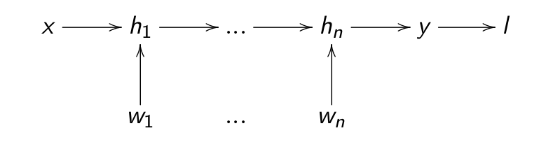
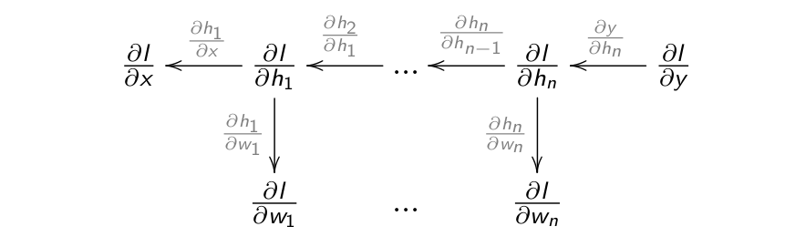
• A feedforward neural network is an acyclic graph of differentiable and parameterized layers.

\mathbf{x} \rightarrow \mathbf{h}_1 \rightarrow \mathbf{h}_2 \rightarrow \ldots \rightarrow \mathbf{h}_n \rightarrow \mathbf{y}

• The backpropagation algorithm is used to assign the gradient of the loss function \mathcal{L}(\theta) to each layer using backward chaining:

\frac{\partial \mathcal{L}(\theta)}{\partial \mathbf{h}_{k-1}} = \frac{\partial \mathcal{L}(\theta)}{\partial \mathbf{h}_{k}} \times \frac{\partial \mathbf{h}_{k}}{\partial \mathbf{h}_{k-1}}

• Stochastic gradient descent is then used to update the parameters of each layer:

\Delta W^k = - \eta \, \frac{\partial \mathcal{L}(\theta)}{\partial W^{k}} = - \eta \, \frac{\partial \mathcal{L}(\theta)}{\partial \mathbf{h}_{k}} \times \frac{\partial \mathbf{h}_{k}}{\partial W^{k}}

4 - Example

MLP example

• Let’s try to solve this non-linear binary classification problem:

MLP example

• We can create a shallow MLP with:

  • Two input neurons x_1, x_2 for the two input variables.

  • Enough hidden neurons (e.g. 20), with a sigmoid or ReLU activation function.

  • One output neuron with the logistic activation function.

  • The cross-entropy (negative log-likelihood) loss function.

• We train it on the input data using the backpropagation algorithm and the SGD optimizer.

MLP example

• Experiment live on https://playground.tensorflow.org/!

Automatic differentiation Deep Learning frameworks

Current:

• Tensorflow https://www.tensorflow.org/ released by Google in 2015 is one of the two standard DL frameworks.

• Keras https://keras.io/ is a high-level Python API over tensorflow (but also theano, CNTK and MxNet) written by Francois Chollet.

• PyTorch http://pytorch.org by Facebook is the other standard framework.

Historical:

• Theano http://deeplearning.net/software/theano/ released by U Toronto in 2010 is the predecessor of tensorflow. Now abandoned.

• Caffe http://caffe.berkeleyvision.org/ by U Berkeley was long the standard library for convolutional networks.

• CNTK https://github.com/Microsoft/CNTK (Microsoft Cognitive Toolkit) is a free library by Microsoft!

• MxNet https://github.com/apache/incubator-mxnet from Apache became the DL framework at Amazon.

Example of a shallow neural network with keras

• Let’s implement the previous MLP using keras.

• We first need to generate the data using scikit-learn:

import sklearn.datasets
X, t = sklearn.datasets.make_circles(n_samples=100, shuffle=True, noise=0.15, factor=0.3)

• We then import tensorflow:

import tensorflow as tf

• The neural network is called a Sequential model in keras:

model = tf.keras.Sequential()

Example of a shallow neural network with keras

• Creating a NN is simply stacking layers in the model. The input layer is just a placeholder for the data:

model.add( tf.keras.layers.Input(shape=(2, )) )

• The hidden layer has 20 neurons, the ReLU activation and takes input from the previous layer:

model.add(
    tf.keras.layers.Dense(
        20, # Number of hidden neurons
        activation='relu' # Activation function
    )
)

• The output layer has 1 neuron with the logistic/sigmoid activation function:

model.add(
    tf.keras.layers.Dense(
        1, # Number of output neurons
        activation='sigmoid' # Soft classification
    )
)

Example of a shallow neural network with keras

• We now choose an optimizer (SGD) with a learning rate \eta = 0.001:

optimizer = tf.keras.optimizers.SGD(lr=0.001)

• We choose a loss function (binary cross-entropy, aka negative log-likelihood):

loss = tf.keras.losses.binary_crossentropy

• We compile the model (important!) and tell it to track the accuracy of the model:

model.compile(
    loss=loss,
    optimizer=optimizer, 
    metrics=tf.keras.metrics.categorical_accuracy
)

Example of a shallow neural network with keras

• Et voilà! The network has been created.

print(model.summary())

Model: "sequential_1"
_________________________________________________________________
Layer (type)                 Output Shape              Param #   
=================================================================
dense (Dense)                (None, 20)                60        
_________________________________________________________________
dense_1 (Dense)              (None, 1)                 21        
=================================================================
Total params: 81
Trainable params: 81
Non-trainable params: 0
_________________________________________________________________
None

Example of a shallow neural network with keras

• We now train the model on the data for 100 epochs using a batch size of 10 and wait for it to finish:

model.fit(X, t, batch_size=10, nb_epoch=100)

• With keras (and the other automatic differentiation frameworks), you only need to define the structure of the network.

• The rest (backpropagation, SGD) is done automatically.

• To make predictions on new data, just do:

model.predict(X_test)