Neurocomputing
Object detection
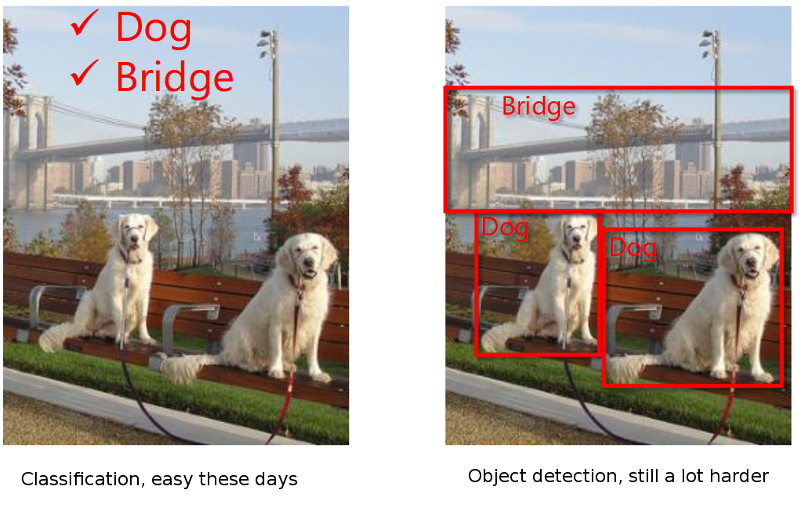
Object recognition vs. object detection
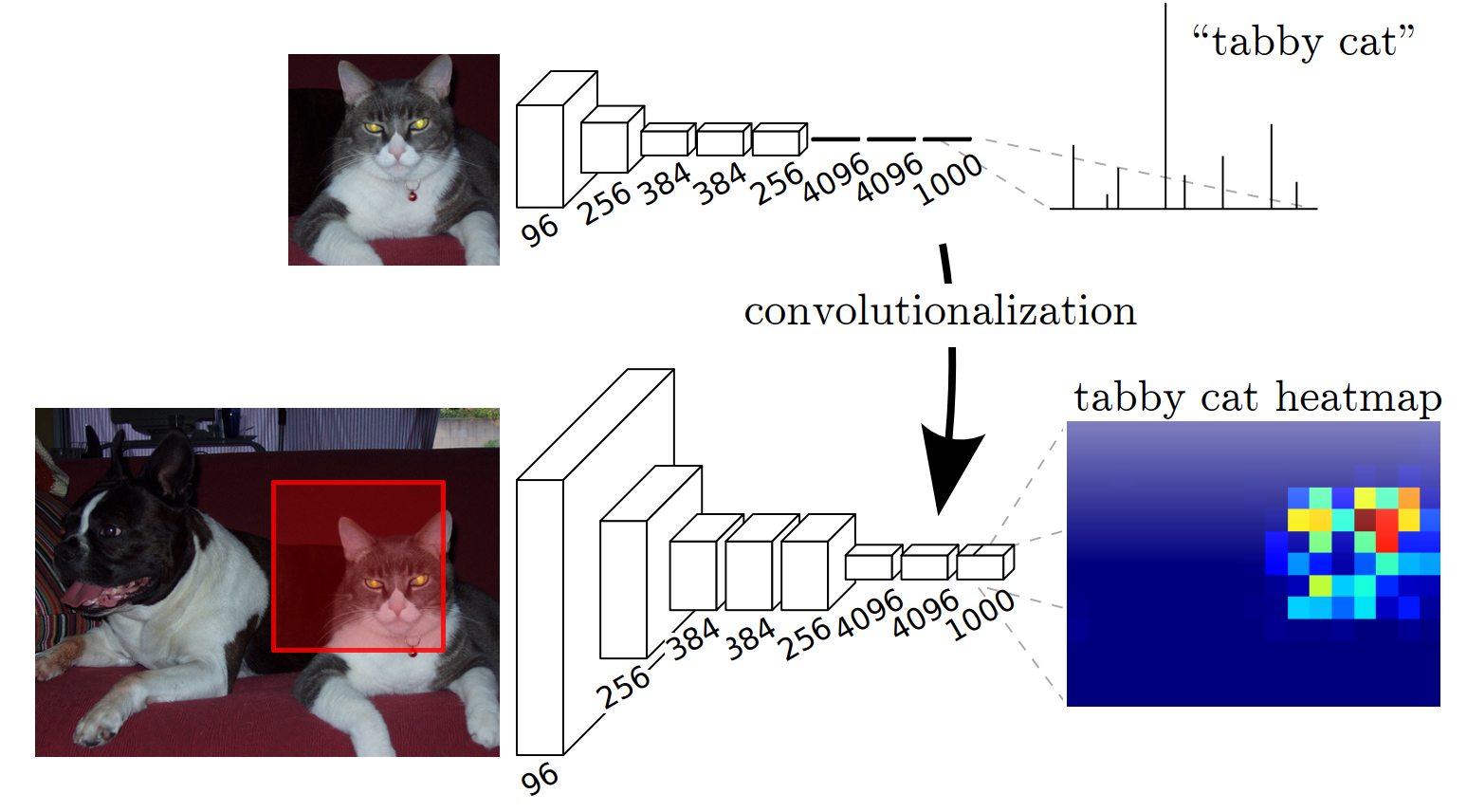
Object detection with heatmaps
A naive and very expensive method is to use a trained CNN as a high-level filter.
The CNN is trained on small images and convolved on bigger images.
The output is a heatmap of the probability that a particular object is present.
PASCAL Visual Object Classes Challenge
The main dataset for object detection is the PASCAL Visual Object Classes Challenge:
20 classes
~10K images
~25K annotated objects
It is both a:
Classification problem, as one has to recognize an object.
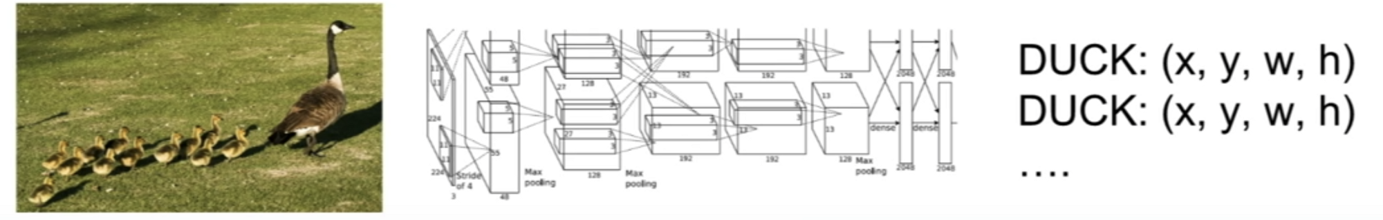
Regression problem, as one has to predict the coordinates (x, y, w, h) of the bounding box.
MS COCO dataset (Common Objects in COntext)

330K images, 80 labels.
Also contains data for semantic segmentation, caption generation, etc.
R-CNN : Regions with CNN features
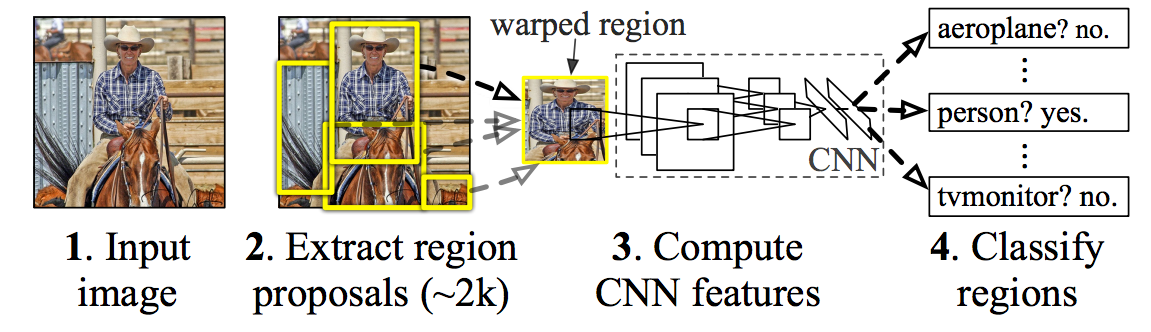
Bottom-up region proposals (selective search) by searching bounding boxes based on pixel info.
Feature extraction using a pre-trained CNN (AlexNet).
Classification using a SVM (object or not; if yes, which one?)
If an object is found, linear regression on the region proposal to generate tighter bounding box coordinates.
R-CNN : Regions with CNN features
- Each region proposal is processed by the CNN, followed by a SVM and a bounding box regressor.
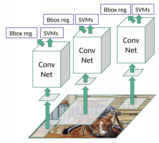
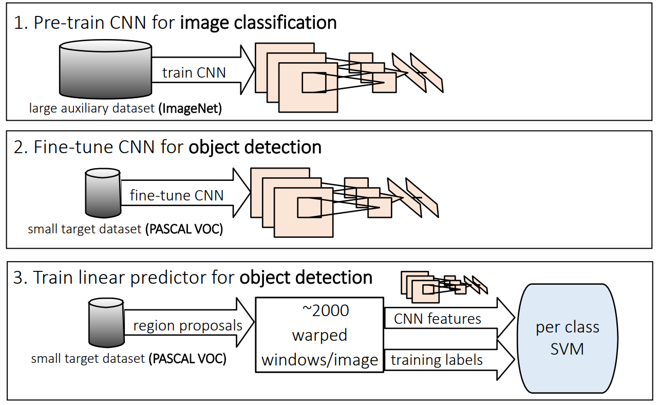
- The CNN is pre-trained on ImageNet and fine-tuned on Pascal VOC.
Fast R-CNN
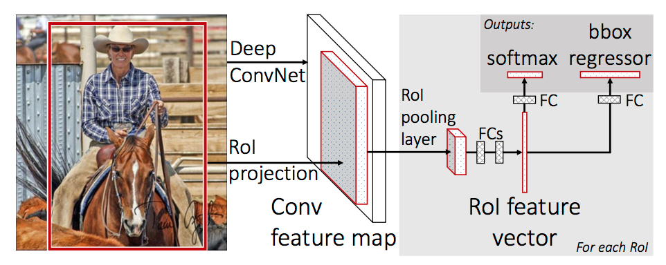
The main drawback of R-CNN is that each of the 2000 region proposals have to go through the CNN: extremely slow.
The idea behind Fast R-CNN is to extract region proposals in higher feature maps and to use transfer learning.
The network first processes the whole image with several convolutional and max pooling layers to produce a feature map.
Each object proposal is projected to the feature map, where a region of interest (RoI) pooling layer extracts a fixed-length feature vector.
Each feature vector is fed into a sequence of FC layers that finally branch into two sibling output layers:
- a softmax probability estimate over the K classes plus a catch-all “background” class.
- a regression layer that outputs four real-valued numbers for each class.
The loss function to minimize is a composition of different losses and penalty terms:
\mathcal{L}(\theta) = \lambda_1 \, \mathcal{L}_\text{classification}(\theta) + \lambda_2 \, \mathcal{L}_\text{regression}(\theta) + \lambda_3 \, \mathcal{L}_\text{regularization}(\theta)
Faster R-CNN
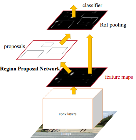
Both R-CNN and Fast R-CNN use selective search to find out the region proposals: slow and time-consuming.
Faster R-CNN introduces an object detection algorithm that lets the network learn the region proposals.
The image is passed through a pretrained CNN to obtain a convolutional feature map.
A separate network is used to predict the region proposals.
The predicted region proposals are then reshaped using a RoI pooling layer which is then used to classify the object and predict the bounding box.
YOLO (You Only Look Once)
(Fast(er)) R-CNN perform classification for each region proposal sequentially: slow.
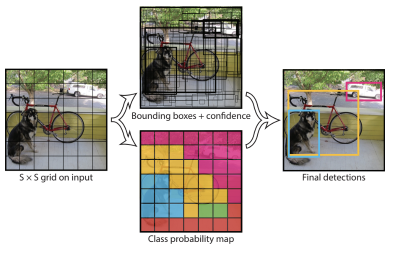
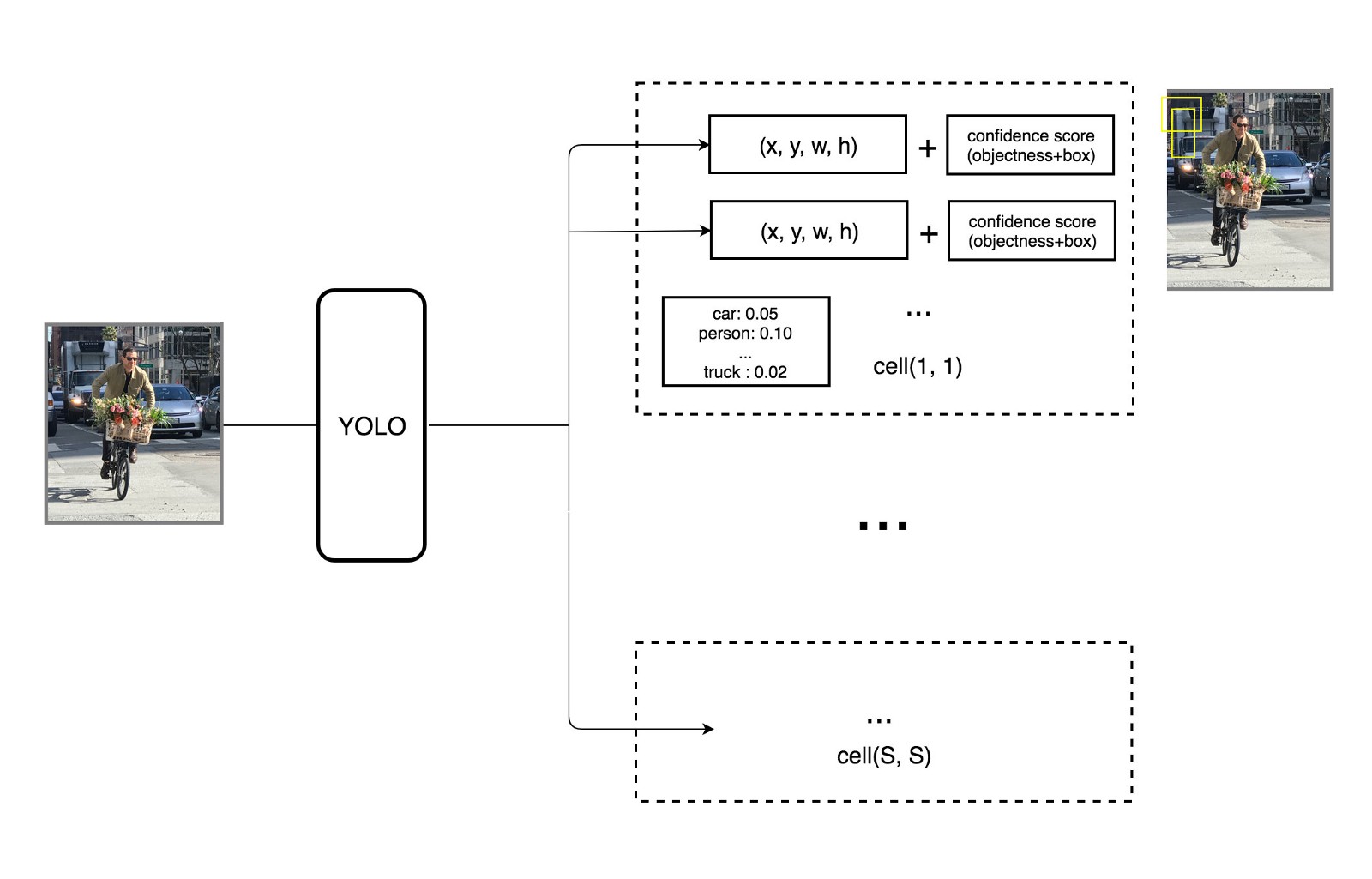
YOLO applies a single neural network to the full image to predict all possible boxes and the corresponding classes.
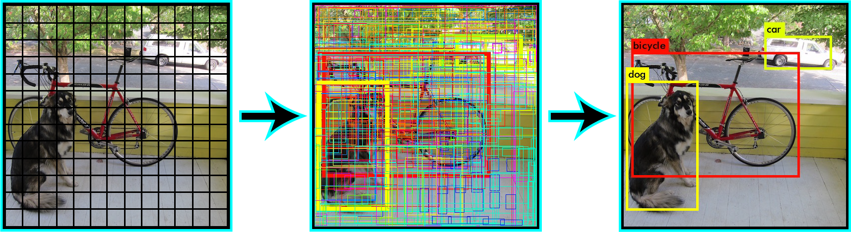
YOLO divides the image into a SxS grid of cells.
Each grid cell predicts a single object, with the corresponding C class probabilities (softmax).
It also predicts the coordinates of B possible bounding boxes (x, y, w, h) as well as a box confidence score.
The SxSxB predicted boxes are then pooled together to form the final prediction.
YOLO (You Only Look Once)
- The yellow box predicts the presence of a person (the class) as well as a candidate bounding box (it may be bigger than the grid cell itself).
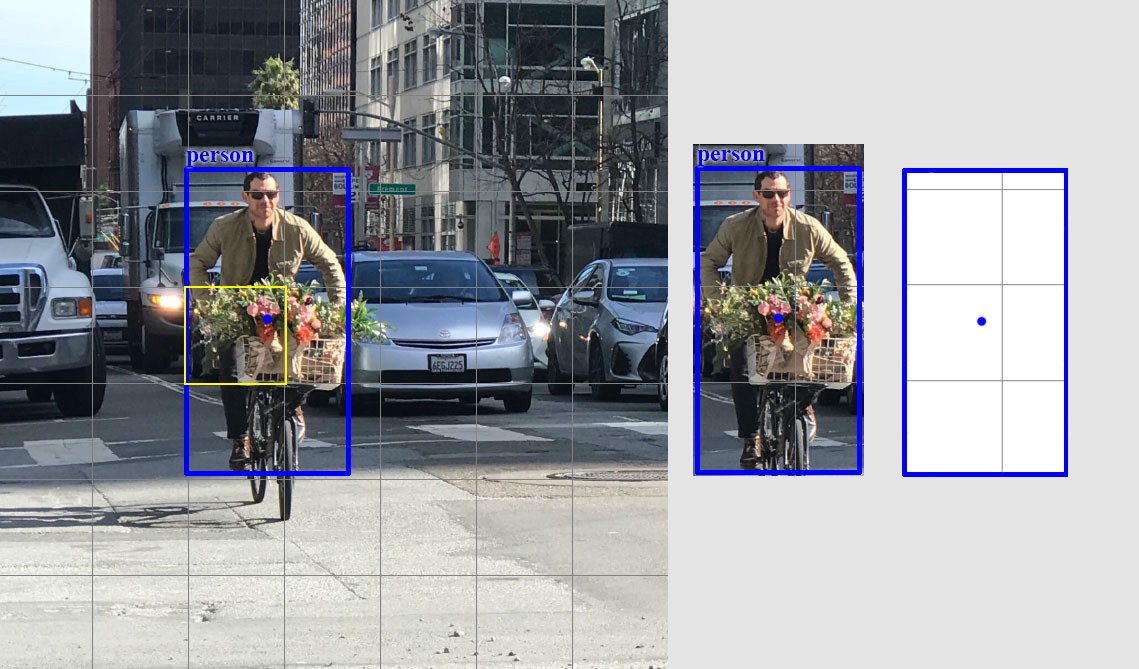
Source: https://medium.com/@jonathan_hui/real-time-object-detection-with-yolo-yolov2-28b1b93e2088
YOLO (You Only Look Once)
- We will suppose here that each grid cell proposes 2 bounding boxes.
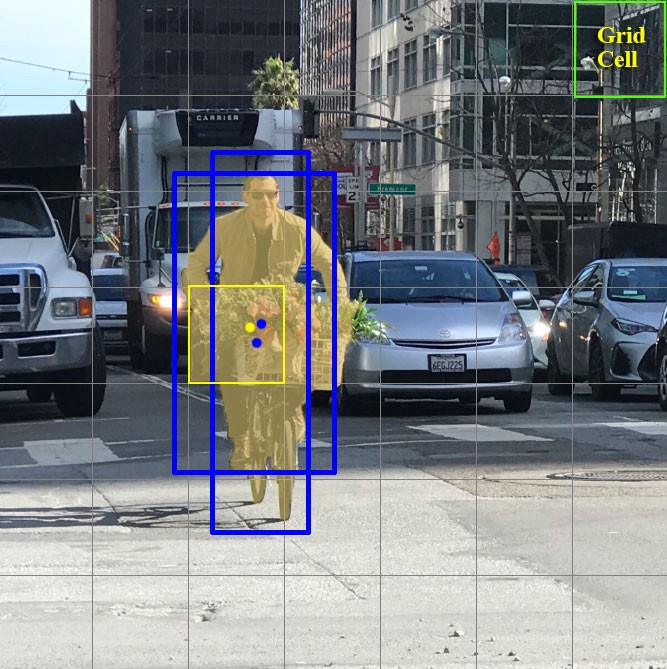
Source: https://medium.com/@jonathan_hui/real-time-object-detection-with-yolo-yolov2-28b1b93e2088
YOLO (You Only Look Once)
Each grid cell predicts a probability for each of the 20 classes, and two bounding boxes (4 coordinates and a confidence score per bounding box).
This makes C + B * 5 = 30 values to predict for each cell.
Source: https://medium.com/@jonathan_hui/real-time-object-detection-with-yolo-yolov2-28b1b93e2088
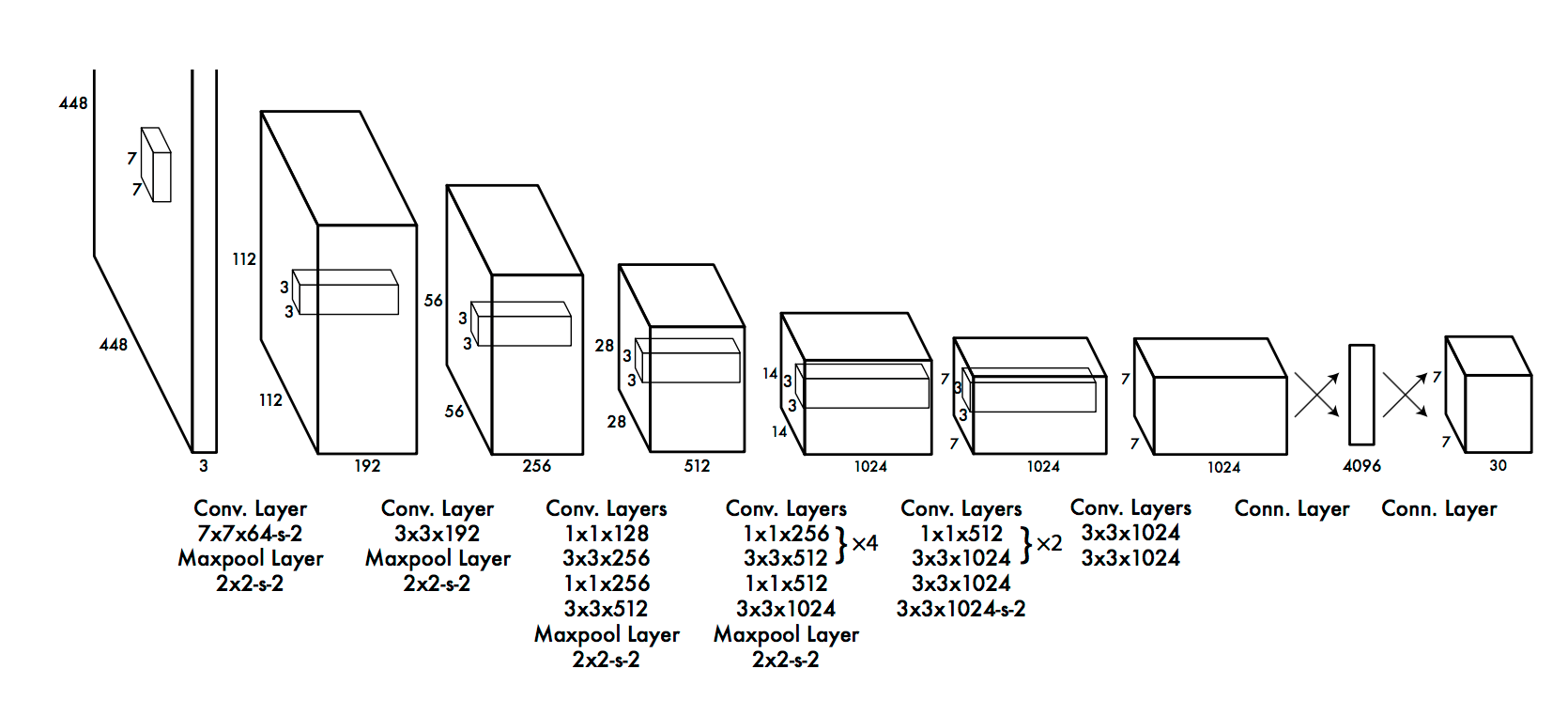
YOLO : CNN architecture
YOLO uses a CNN with 24 convolutional layers and 4 max-pooling layers to obtain a 7x7 grid.
The last convolution layer outputs a tensor with shape (7, 7, 1024). The tensor is then flattened and passed through 2 fully connected layers.
The output is a tensor of shape (7, 7, 30), i.e. 7x7 grid cells, 20 classes and 2 boundary box predictions per cell.
YOLO : confidence score
The 7x7 grid cells predict 2 bounding boxes each: maximum of 98 bounding boxes on the whole image.
Only the bounding boxes with the highest class confidence score are kept.
\text{class confidence score = box confidence score * class probability}
- In practice, the class confidence score should be above 0.25 to be retained.
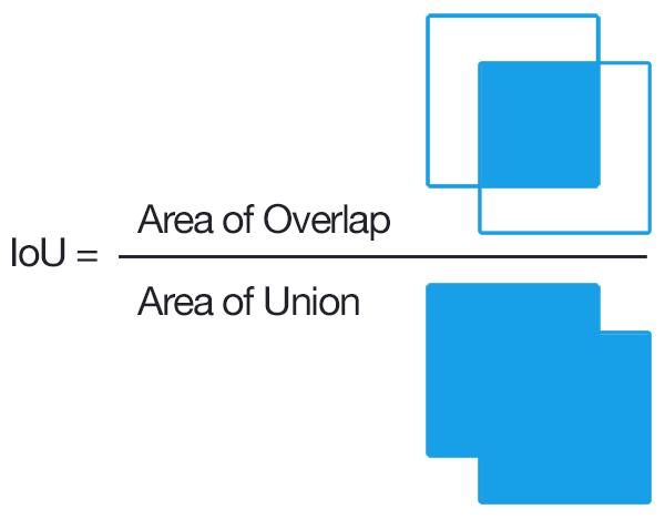
YOLO : Intersection over Union (IoU)
To ensure specialization, only one bounding box per grid cell should be responsible for detecting an object.
During learning, we select the bounding box with the biggest overlap with the object.
This can be measured by the Intersection over the Union (IoU).
YOLO : Training on PASCAL VOC

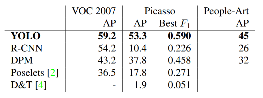
YOLO was trained on PASCAL VOC (natural images) but generalizes well to other datasets (paintings…).
Runs real-time (60 fps) on a NVIDIA Titan X.
Faster and more accurate versions of YOLO have been developed: YOLO9000, YOLOv3, YOLOv4, YOLOv5…
SSD: Single-Shot Detector
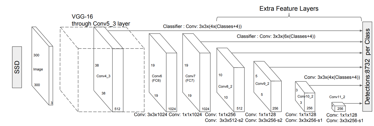
The idea of SSD is similar to YOLO, but:
- faster
- more accurate
- not limited to 98 objects per scene
- multi-scale
Contrary to YOLO, all convolutional layers are used to predict a bounding box, not just the final tensor.
- Skip connections.
This allows to detect boxes at multiple scales (pyramid).
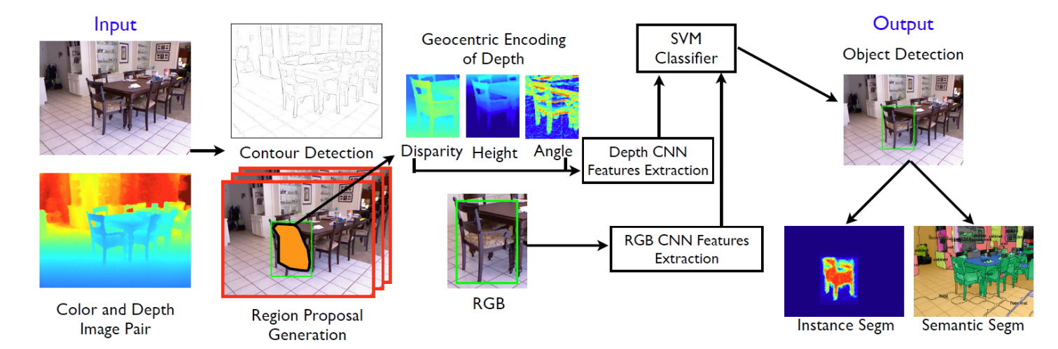
R-CNNs on RGB-D images
It is also possible to use depth information (e.g. from a Kinect) as an additional channel of the R-CNN.
The depth information provides more information on the structure of the object, allowing to disambiguate certain situations (segmentation).
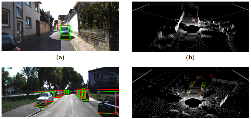
VoxelNet
- Lidar point clouds can also be used for detecting objects, for example VoxelNet trained on the KITTI dataset.
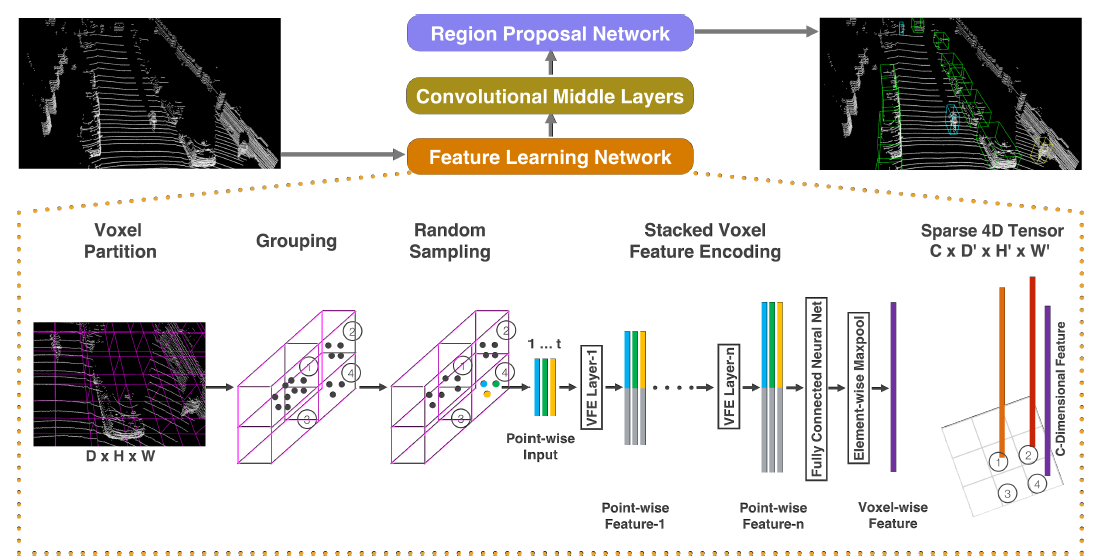
VoxelNet
Source: https://medium.com/@SmartLabAI/3d-object-detection-from-lidar-data-with-deep-learning-95f6d400399a
Metrics for object detection
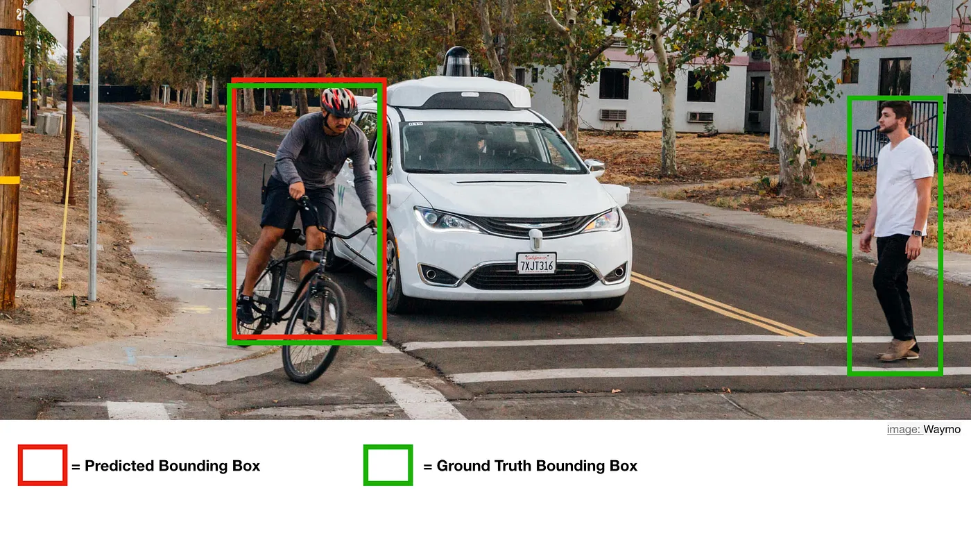
How do we measure the “accuracy” of an object detector? The output is both a classification and a regression.
Not only must the predicted class be correct, but the predicted bounding box must overlap with the ground truth, i.e. have an high IoU.
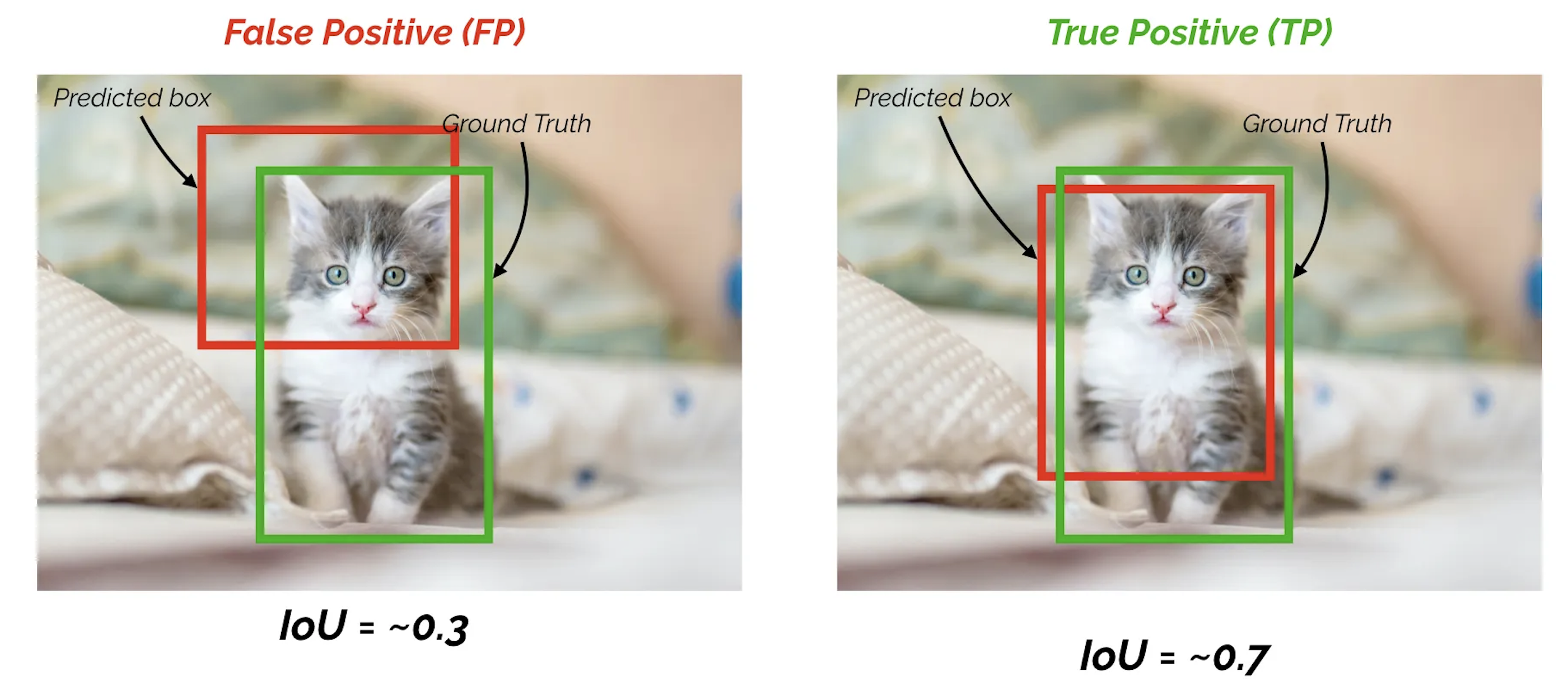
Source: https://towardsdatascience.com/map-mean-average-precision-might-confuse-you-5956f1bfa9e2
Metrics for object detection
The accuracy of an object detector depends on a threshold for the IoU, for example 0.5.
A prediction is correct if the predicted class is correct and the IoU is above the threshold.
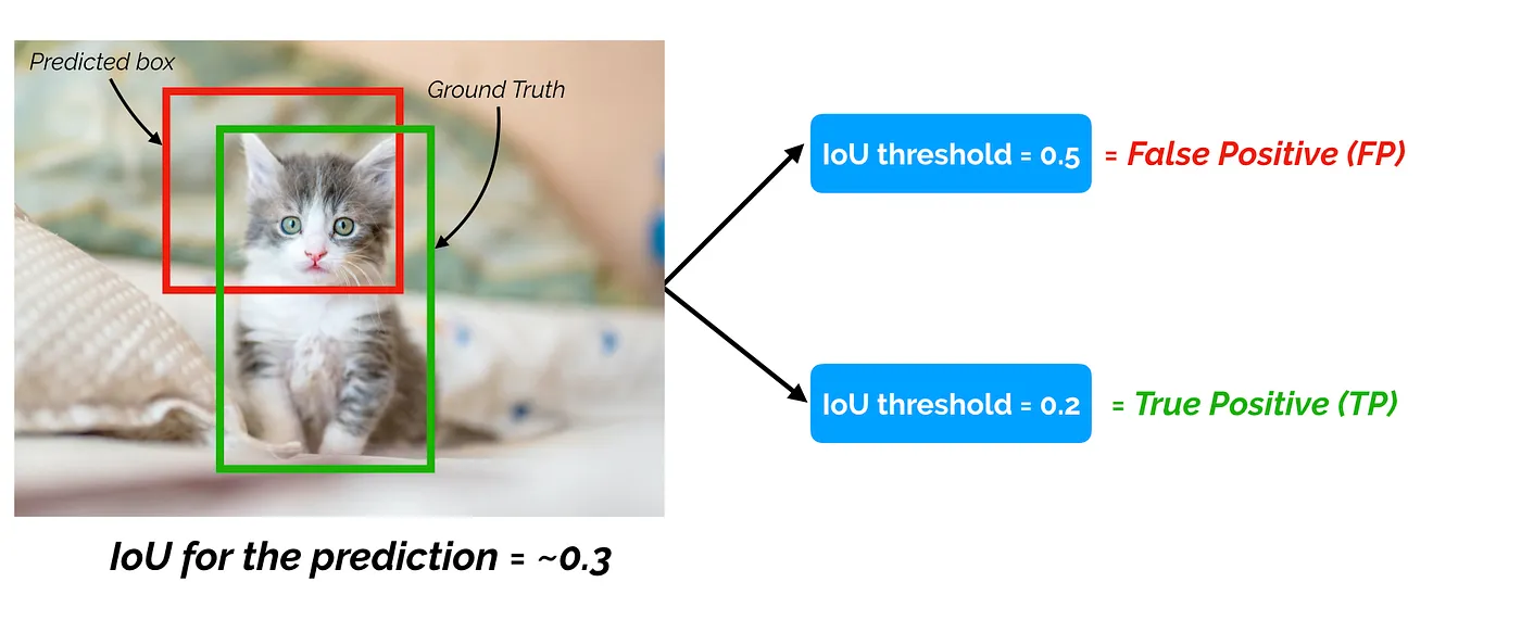
Source: https://towardsdatascience.com/map-mean-average-precision-might-confuse-you-5956f1bfa9e2
Precision and recall
- For a given class (e.g. “human”), we can compute the binary precision and recall values:
P = \frac{\text{TP}}{\text{TP} + \text{FP}} \;\; R = \frac{\text{TP}}{\text{TP} + \text{FN}}
P = when something is detected, is it correct? R = if something exists, is it detected?
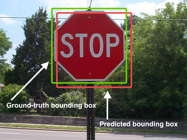
In the image below, we have one TP, one FN, zero FP and an undefined number of TN:
P = \frac{\text{1}}{\text{1} + \text{0}} = 1\;\; R = \frac{\text{1}}{\text{1} + \text{1}} = 0.5
Source: https://towardsdatascience.com/map-mean-average-precision-might-confuse-you-5956f1bfa9e2
mAP: mean average precision
- Let’s now compute the precision-recall curve over 7 images, with 15 ground truth boxes and 24 predictions.
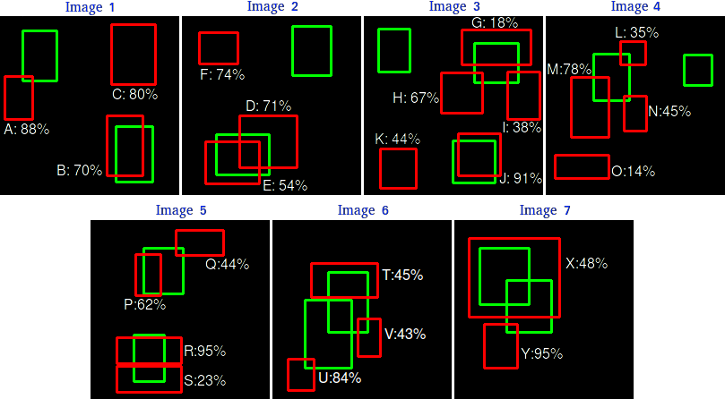
- Each prediction has a confidence score for the classification, and is either a TP or FP (depending on the IoU threshold).
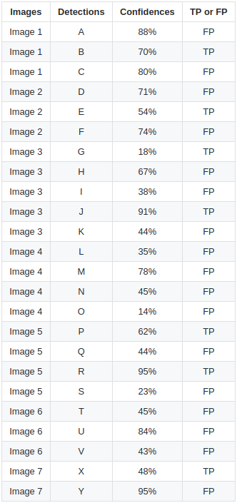
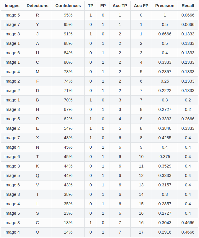
mAP: mean average precision
- Let’s now sort the predictions with a decreasing confidence score and incrementally compute the prediction and recall:
P = \frac{\text{TP}}{\text{TP} + \text{FP}} R = \frac{\text{TP}}{\text{TP} + \text{FN}}
We just accumulate the number of TP and FP over the 24 predictions.
Note that
TP + FNis the number of ground truths and is constant (15), so the recall will increase.This equivalent to setting a high threshold for the confidence score and progressively decreasing it.
mAP: mean average precision
- If we plot the precision x recall curve (PR curve) for the 24 predictions, we obtain:
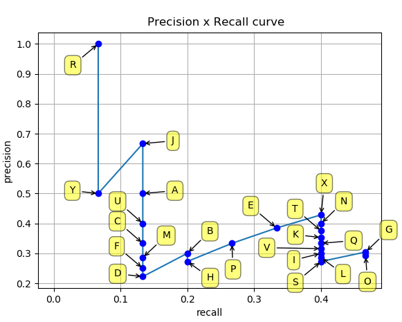
- The precision globally decreases with the recall, as we use predictions with lower confidence scores, but there are some oscillations.
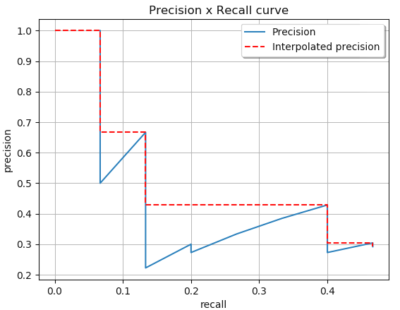
mAP: mean average precision
To get rid of these oscillations, we interpolate the precision by taking maximal precision value for higher recall (left).
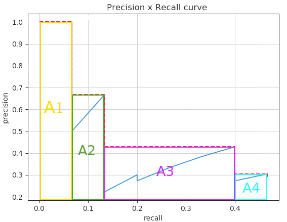
We can then easily integrate this curve by computing the area under the curve (AUC, right), what defines the average precision (AP).
\text{AP} = \sum_n (R_{n} - R_{n-1}) \, P_n
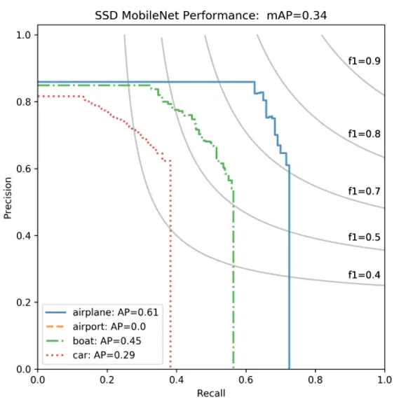
mAP: mean average precision
A good detector sees its precision decreases not that much when the recall increases, i.e. when it is still correct when it increasingly detects objects.
The ideal detector has an AP of 1.
When averaging the AP over the classes, one obtains the mean average precision (mAP):
\text{mAP} = \dfrac{1}{N_\text{classes}} \, \sum_{i=1}^{N_\text{classes}} \, AP_i
One usually reports the mAP value with the IoU threshold, e.g.
mAP@0.5.mAP is a better trade-off between precision and recall than the F1 score.
scikit-learnis your friend:
mAP = sklearn.metrics.average_precision_score(t, y, average="micro")