Neurocomputing
Diffusion Probabilistic Models
1 - Denoising Diffusion Probabilistic Model (DDPM)

Generative modeling
Generative modeling consists in transforming a simple probability distribution (e.g. Gaussian) into a more complex one (e.g. images).
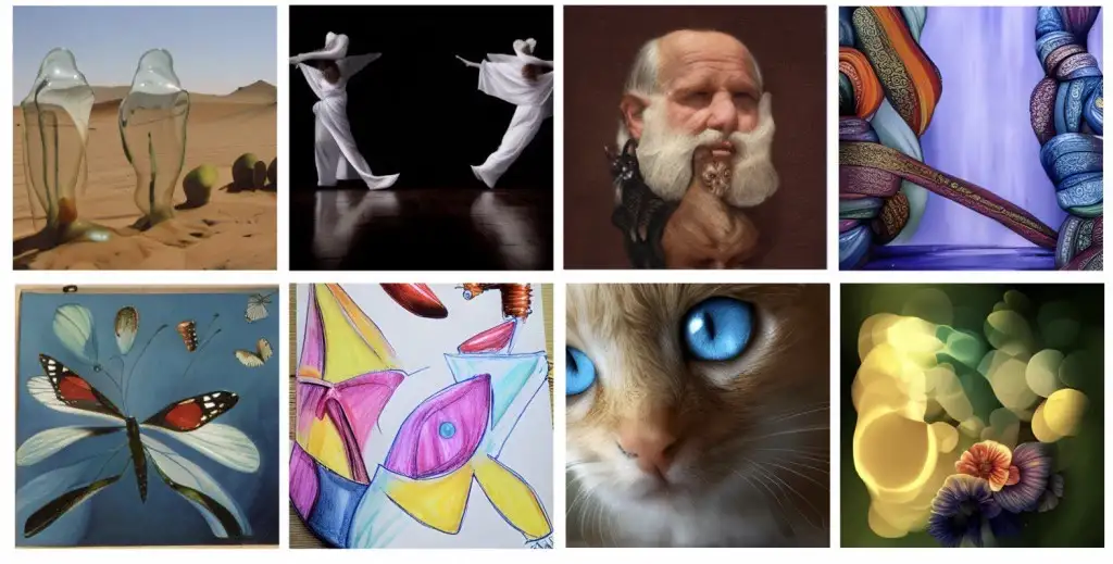
Learning this model allows to easily sample complex images.
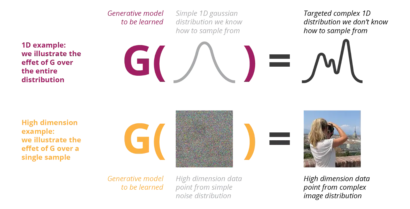
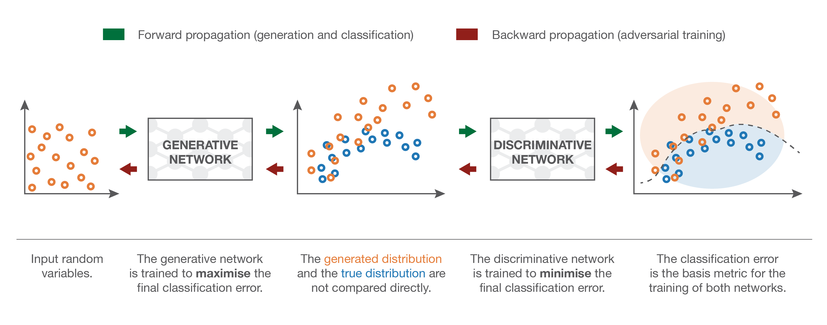
VAE and GAN transform simple noise into complex distributions
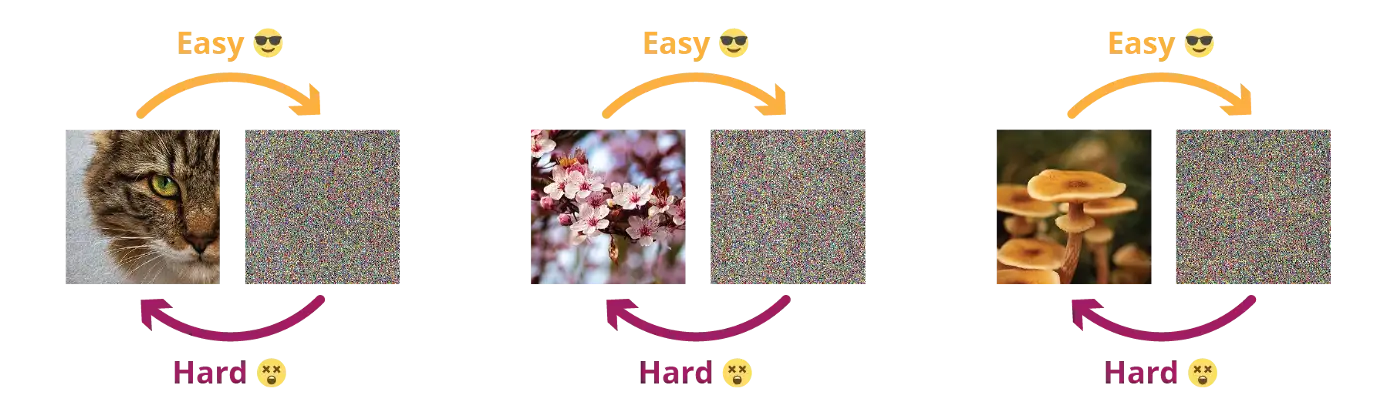
Destroying information is easier than creating it
The task of the generators in GAN or VAE is very hard: going from noise to images in a few layers.
The other direction is extremely easy.
Diffusion process
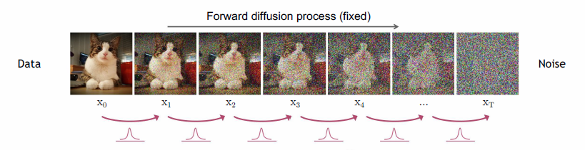
The forward diffusion process iteratively destructs all information in the image through a Markov chain that adds white noise.
A Markov chain implies that each step is independent and governed by a probability distribution q(x_t | x_{t-1}).
Stochastic processes can destroy information
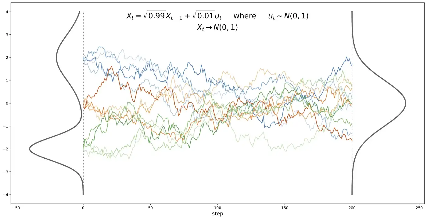
- Iteratively adding normal noise to a signal creates a stochastic differential equation (SDE), such as the Ornstein–Uhlenbeck (OU) stochastic process.
\begin{aligned} \text{discrete:} \qquad& x_t = \sqrt{1 - \beta_t} \, x_{t-1} + \sqrt{\beta_t} \, \epsilon \\ & \qquad\qquad\text{where} \qquad \epsilon \sim \mathcal{N}(0, 1) \\ &\\ \text{continuous:} \qquad & dx = - \dfrac{1}{2} \, \beta(t) \, x \, dt + \sqrt{\beta(t)} \, dW \\ \end{aligned}
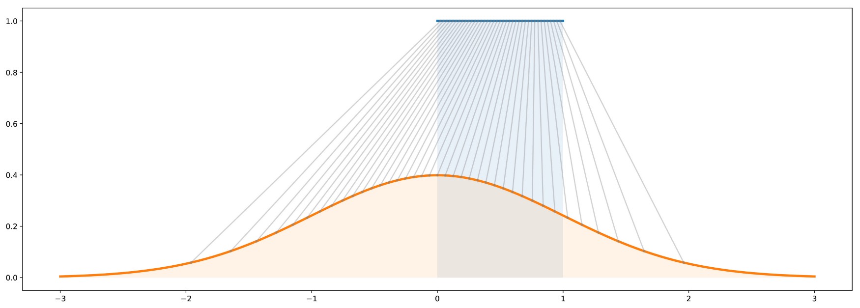
- Any probability distribution converges to a normal distribution when following the OU process.
- The Focker-Planck equation is a general form of the OU process (drift + diffusion), hence the name:
dx = \underbrace{\mu(x, t) \, dt}_{\text{drift}} + \underbrace{\sigma(x, t) \, dW}_{\text{diffusion}}
Probabilistic diffusion models
- It should be possible to reverse each diffusion step by removing the noise using a sort of denoising autoencoder.
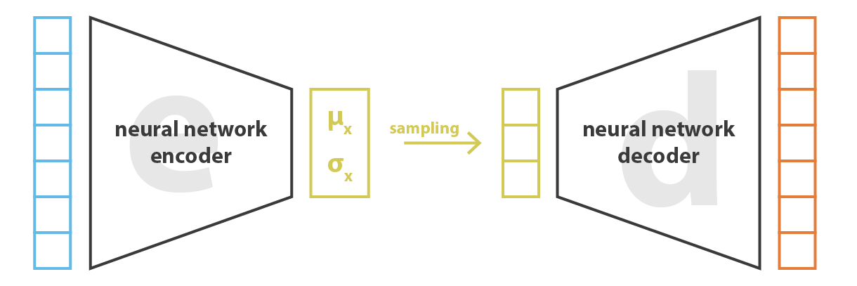
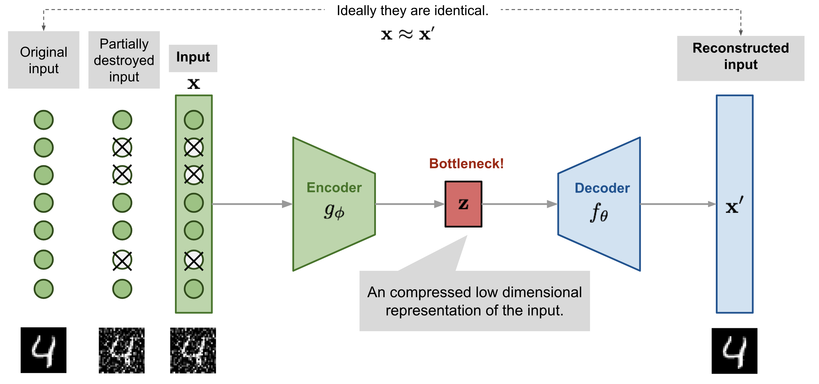
Reminder: Denoising autoencoder
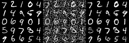
- A denoising autoencoder (DAE) is trained with noisy inputs but perfect desired outputs. It learns to suppress that noise.
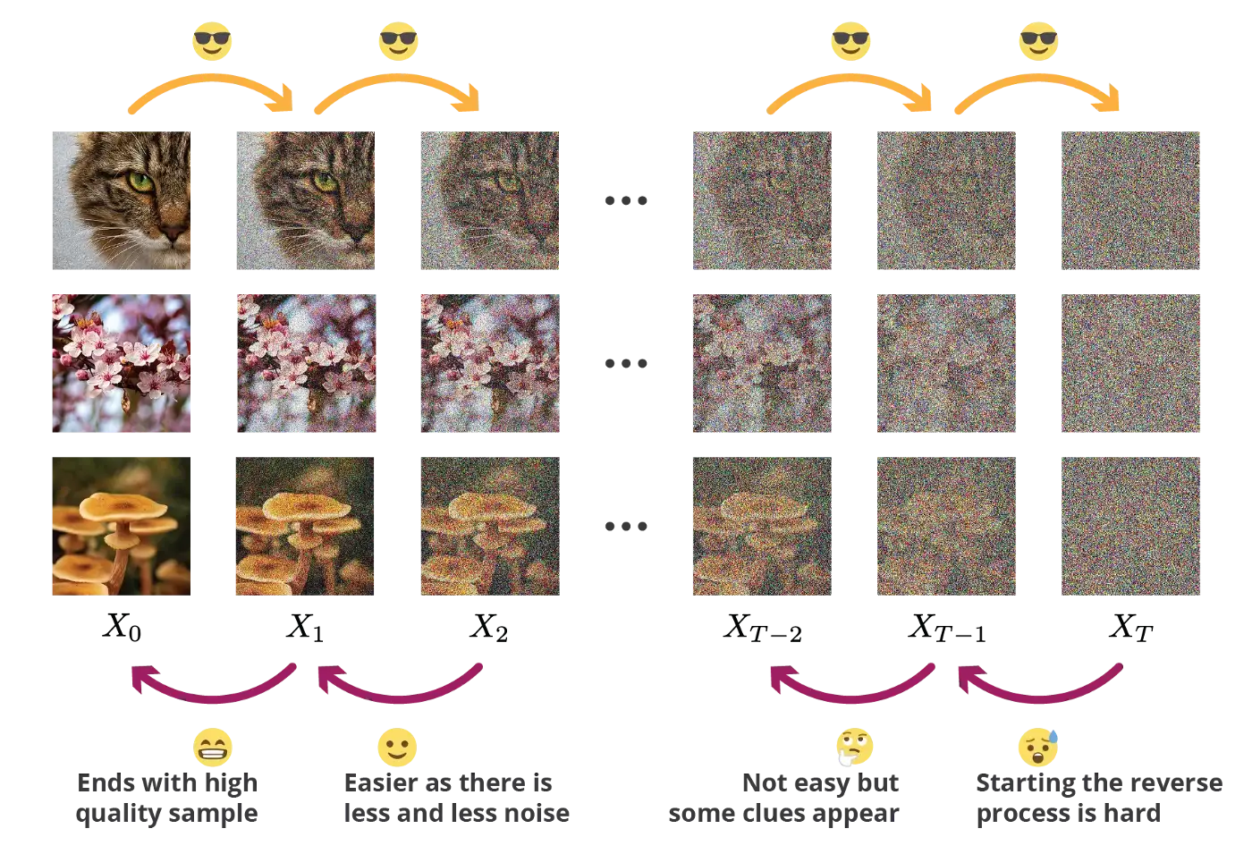
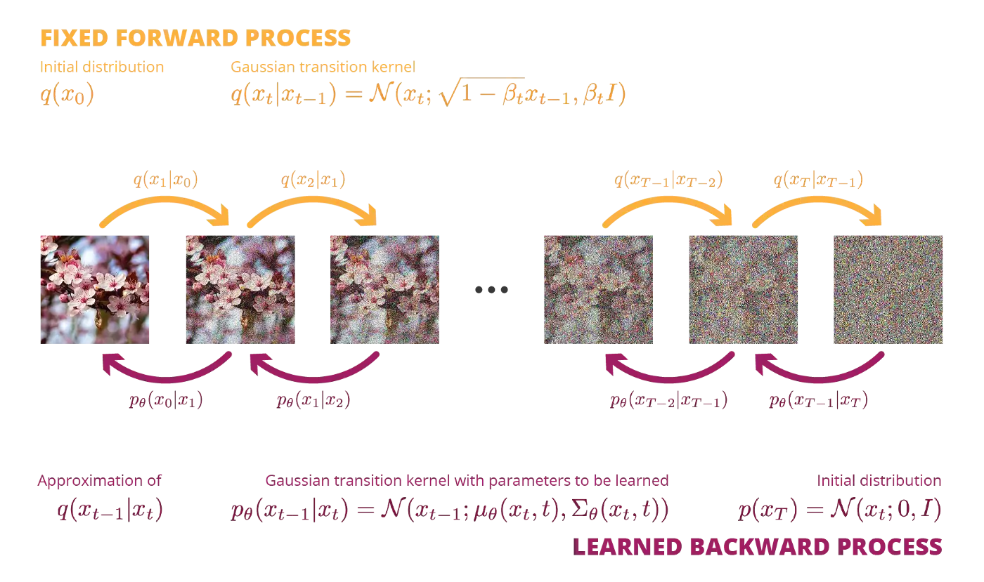
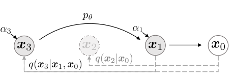
Forward Diffusion process
The forward process iteratively corrupts the image using q(x_t | x_{t-1}) for T steps (e.g. T=1000).
The goal is to learn a reverse process p_\theta(x_{t-1} | x_t) that approximates the true posterior q(x_{t-1} | x_t).
Forward Diffusion process
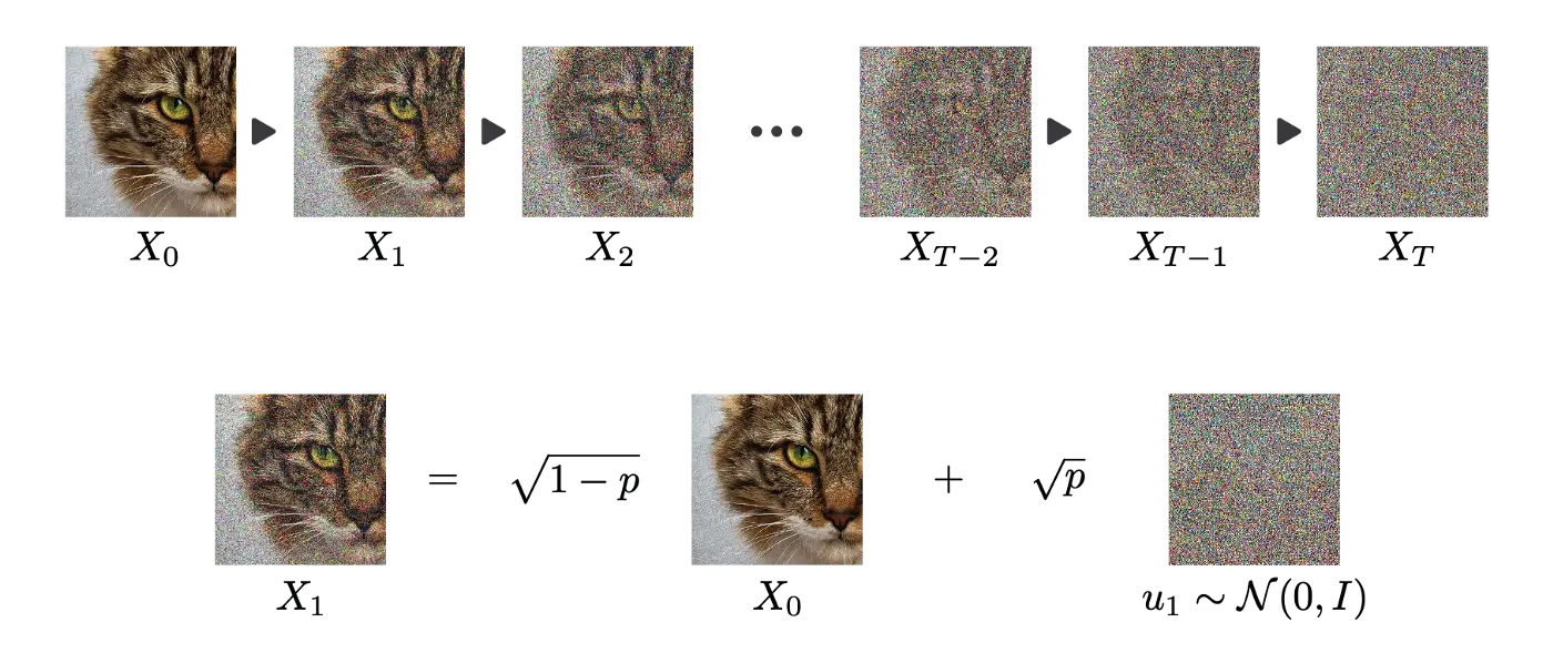
- The forward diffusion process iteratively adds Gaussian noise with a fixed variance schedule \beta_t:
x_t = \sqrt{1 - \beta_t} \, x_{t-1} + \sqrt{\beta_t} \, \epsilon \;\; \text{where} \; \epsilon \sim \mathcal{N}(0, I)
- It is equivalent to say that we sample x_t from a conditional normal distribution.
q(x_t | x_{t-1}) = \mathcal{N}(\mu_t = \sqrt{1 - \beta_t} \, x_{t-1}, \Sigma_t^2 = \beta_t \, I)
\mu_t = \sqrt{1 - \beta_t} \, x_{t-1} is the mean of the distribution, \Sigma_t^2 = \beta_t \, I its variance.
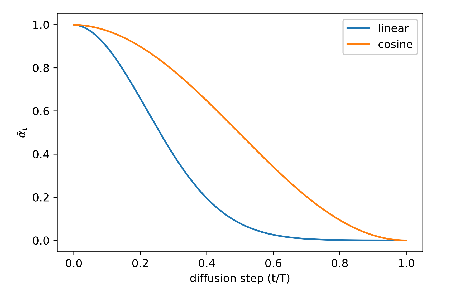
The parameter \beta_t is annealed with a decreasing schedule, as adding more noise at the end does not destroy much more information.
Forward Diffusion process
- Nice property: each image x_t is also a noisy version of the original image x_0:
q(x_t | x_{0}) = \mathcal{N}(\sqrt{\bar{\alpha}_t} \, x_0 , (1 - \bar{\alpha}_t) \, I) x_t = \sqrt{\bar{\alpha}_t} \, x_0 + \sqrt{1 - \bar{\alpha}_t} \, \epsilon_t \;\; \text{where} \; \epsilon_t \sim \mathcal{N}(0, I)
with \alpha_t = 1 - \beta_t and \bar{\alpha}_t = \prod_{s=1}^t \alpha_s only depending on the history of \beta_t.
Adding Gaussian noise to Gaussian noise is still Gaussian noise.
We do not need to perform t noising steps on x_0 to obtain x_t!
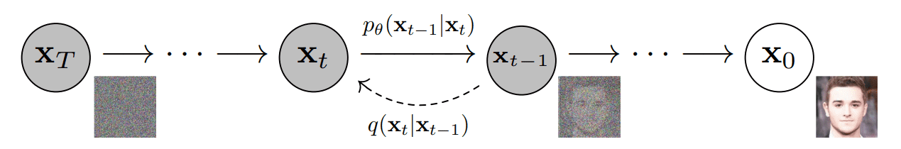
Reverse diffusion model
- The goal of the reverse diffusion process is to find a parameterized model p_\theta explaining the sequence of images backwards in time:
p_\theta(x_{0:T}) = p(x_T) \, \prod_{t=1}^T p_\theta(x_{t-1} | x_t)
where:
p_\theta(x_{t-1} | x_t) = \mathcal{N}(\mu_\theta(x_t, t), \Sigma_\theta(x_t, t))
- The reverse process is also normally distributed, given that the noise \beta_t is not too big.
Denoising Probabilistic Diffusion Model
- By doing some Bayesian inference on the true posterior q(x_{t-1} | x_t) = \mathcal{N}(\mu_t, \Sigma_t), Ho et al. (2020) could show that:
\begin{cases} \mu_t = \dfrac{1}{\sqrt{\alpha_t}} \, (x_t - \dfrac{1-\alpha_t}{\sqrt{1 - \bar{\alpha}_t}} \, \epsilon_t)\\ \\ \Sigma_t = \dfrac{1 - \bar{\alpha}_{t-1}}{1 - \bar{\alpha}_{t}} \beta_t \, I = \bar{\beta}_t \, I \\ \end{cases}
- The reverse variance only depends on the schedule of \beta_t, it can be pre-computed.
Denoising Probabilistic Diffusion Model
- The reverse model p_\theta(x_{t-1} | x_t) only need to approximate the mean:
\mu_\theta(x_t, t) = \dfrac{1}{\sqrt{\alpha_t}} \, (x_t - \dfrac{1-\alpha_t}{\sqrt{1 - \bar{\alpha}_t}} \, \epsilon_\theta(x_t, t))
x_t is an input to the model, it does not have to predicted.
All we need to learn is the noise \epsilon_\theta(x_t, t) \approx \epsilon_t that was added to the original image x_0 to obtain x_t:
x_t = \sqrt{\bar{\alpha}_t} \, x_0 + \sqrt{1 - \bar{\alpha}_t} \, \epsilon_t
Denoising Probabilistic Diffusion Model
- We want to predict the added noise in the image space:
\epsilon_\theta(x_t, t) = \epsilon_\theta(\sqrt{\bar{\alpha}_t} \, x_0 + \sqrt{1 - \bar{\alpha}_t} \, \epsilon_t, t) \approx \epsilon_t
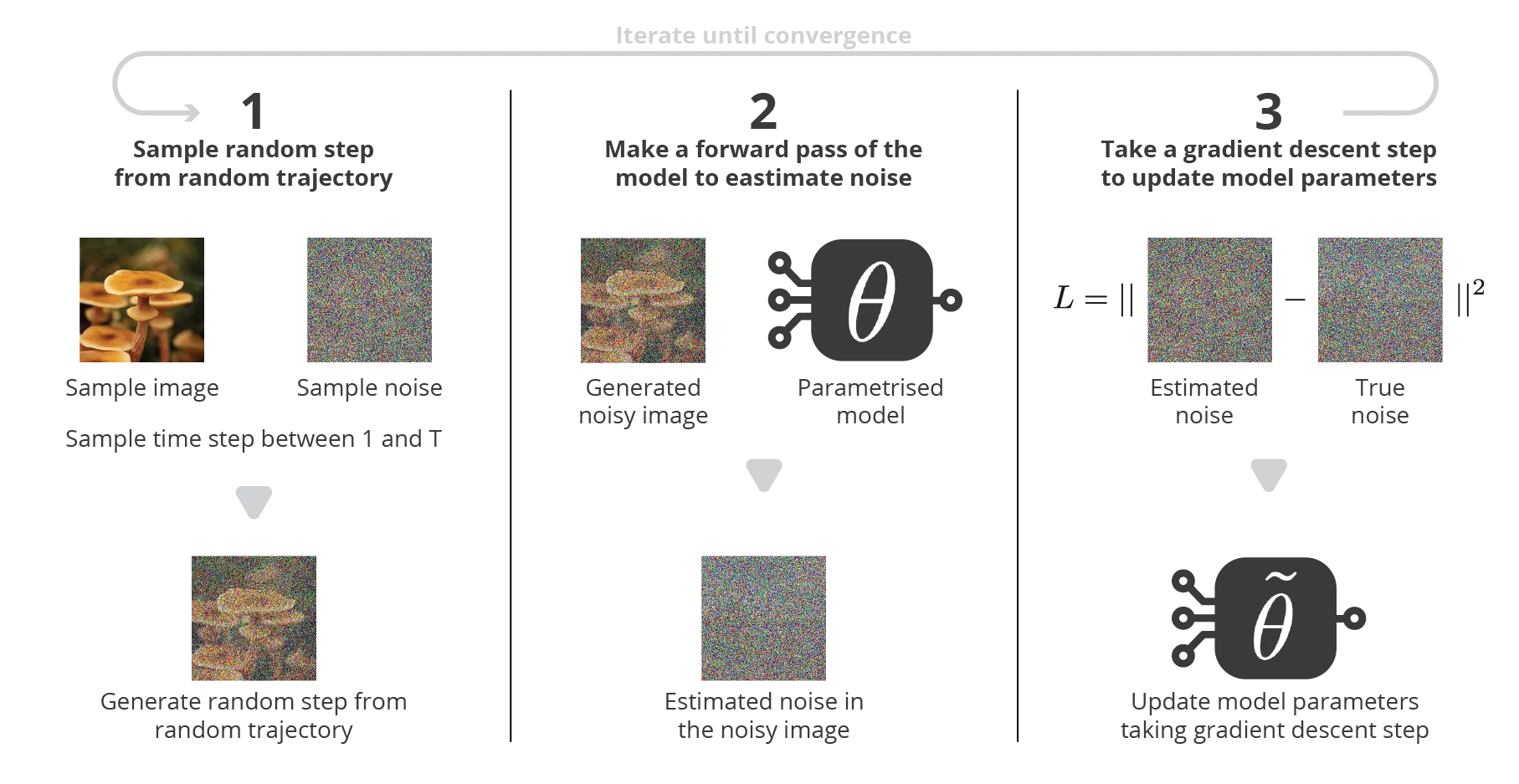
- We can simply minimize the mse with the true noise:
\begin{aligned} \mathcal{L}(\theta) &= \mathbb{E}_{t \sim [1, T], x_0, \epsilon_t} [(\epsilon_t - \epsilon_\theta(x_t, t))^2] \\ &= \mathbb{E}_{t \sim [1, T], x_0, \epsilon_t} [(\epsilon_t - \epsilon_\theta(\sqrt{\bar{\alpha}_t} \, x_0 + \sqrt{1 - \bar{\alpha}_t} \, \epsilon_t, t) )^2] \\ \end{aligned}
- We only need to sample an image x_0, a time step t, a noise \epsilon_t \sim \mathcal{N}(0, I), predict the noise \epsilon_\theta(x_t, t) and minimize the mse!
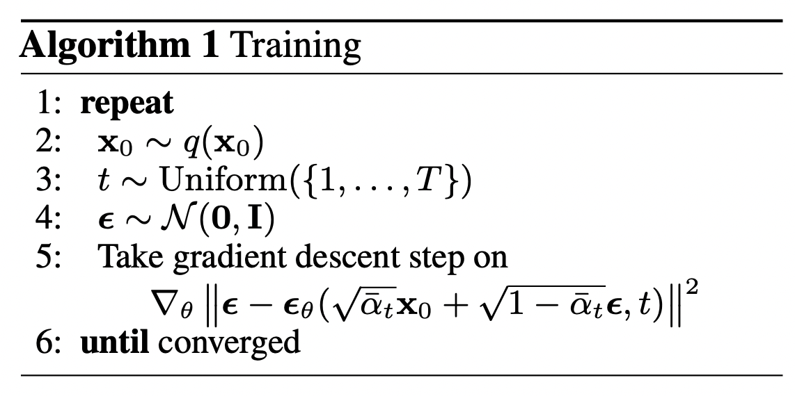
Denoising Probabilistic Diffusion Model
- Training can be done on individual samples, no need for the whole Markov chain to create the minibatches.
DDPM backbone
- The neural network used for the reverse diffusion is usually some kind of U-net, with attentional layers, or even a vision Transformer.
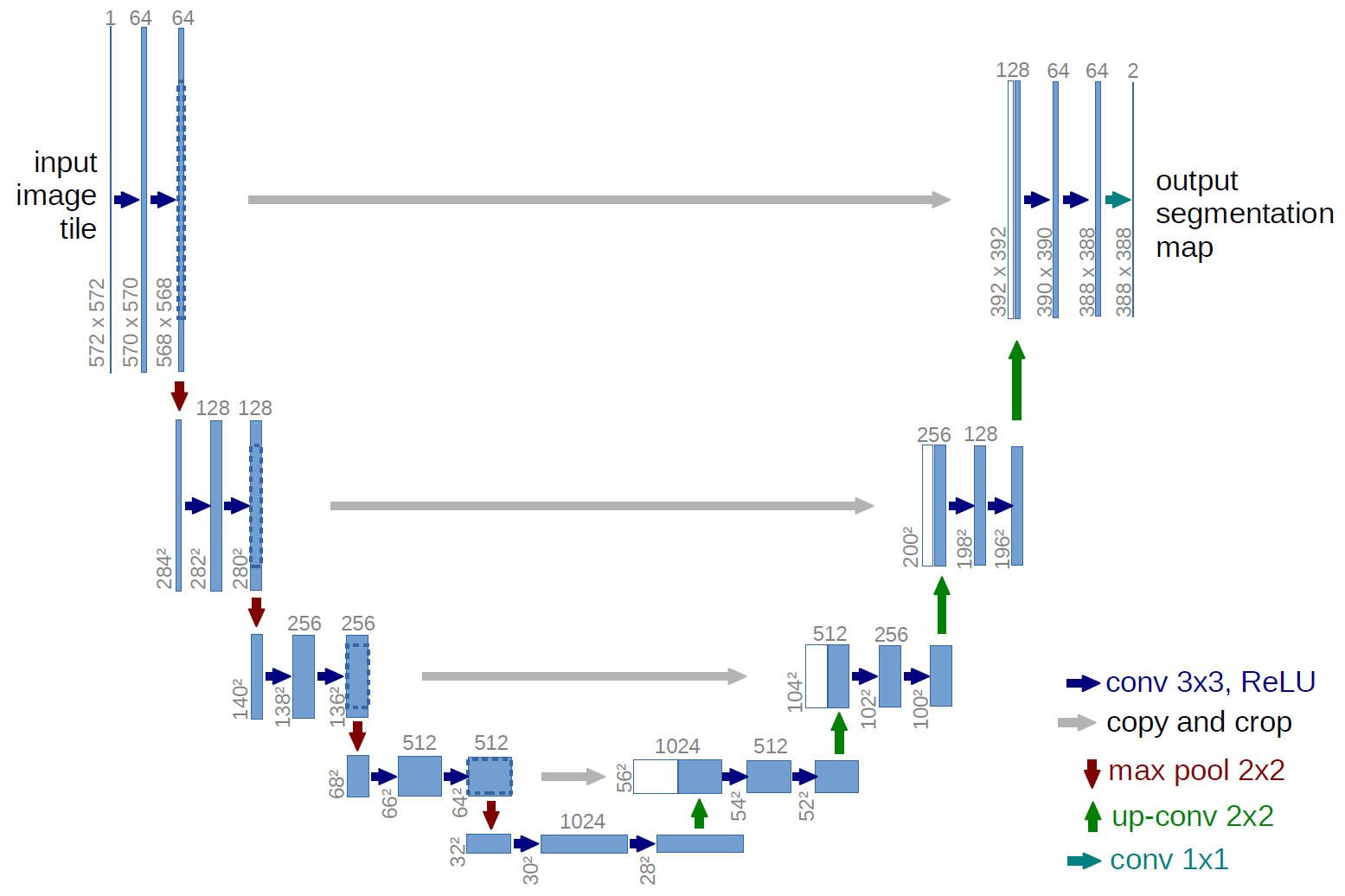
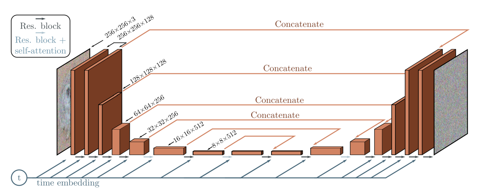
- A time embedding for the time index t is necessary. It is usually added to each layer of the U-Net.
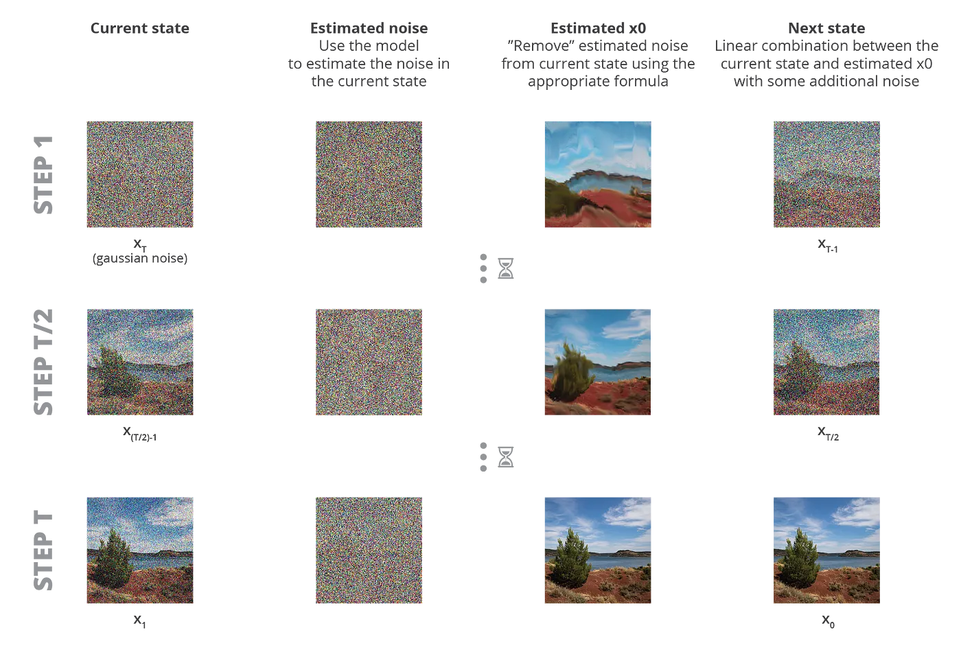
DDPM sampler
- The reverse diffusion occurs iteratively backwards in time (1000 steps) by sampling the posterior:
p_\theta(x_{t-1} | x_t) = \mathcal{N}(\mu_\theta(x_t, t), \bar{\beta}_t \, I)
x_{t-1} = \dfrac{1}{\sqrt{\alpha_t}} \, (x_t - \dfrac{1-\alpha_t}{\sqrt{1 - \bar{\alpha}_t}} \, \epsilon_\theta(x_t, t)) + \bar{\beta}_t \, \epsilon
The last step x_1 \rightarrow x_0 can be done deterministically.
It is possible to use less iterations (200) by taking bigger steps, but this stays expensive and generates lower quality images.
Denoising Probabilistic Diffusion Model

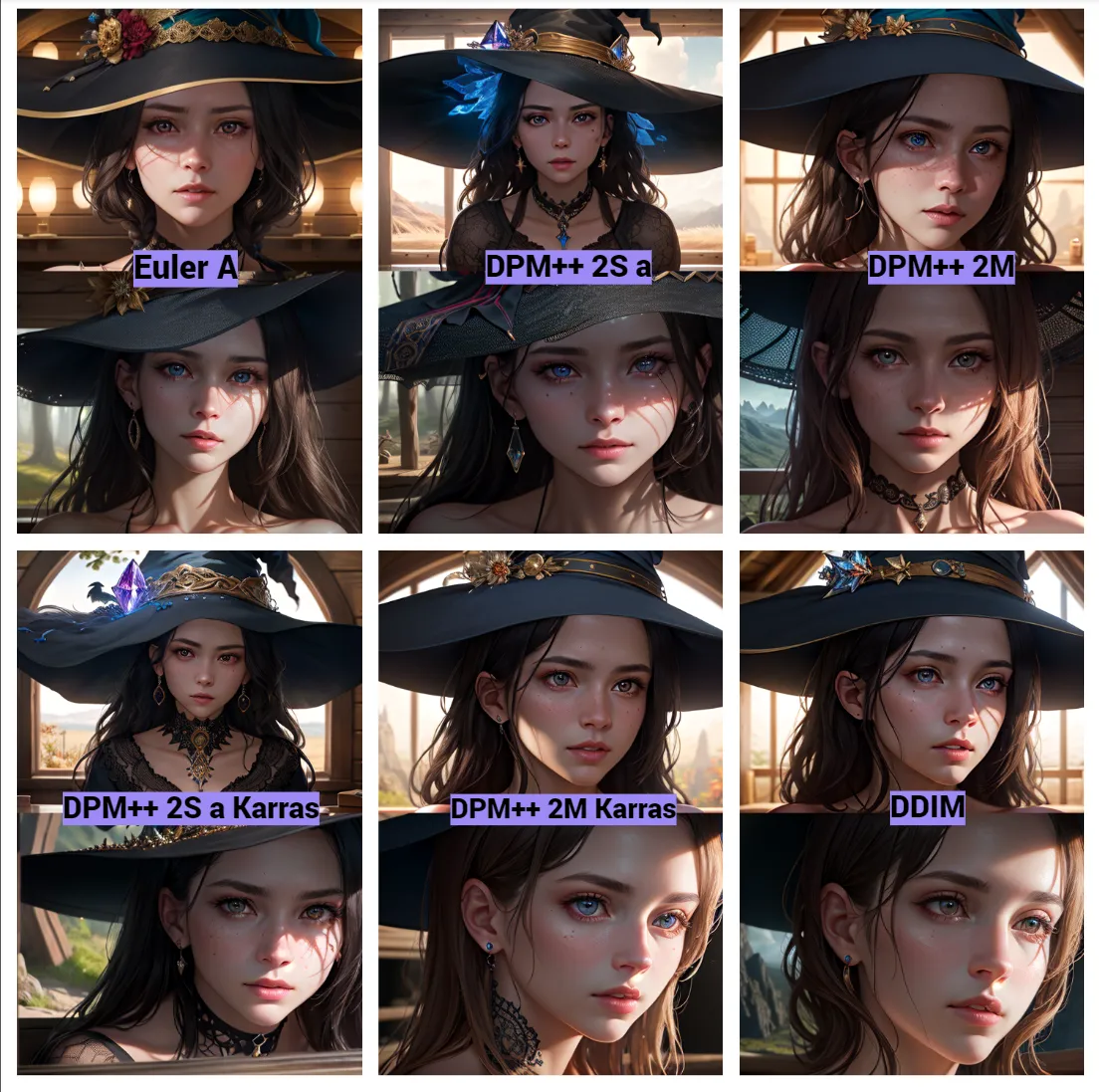
Modern samplers
- The equivalent SDE is:
dx = \left[-\frac{1}{2}\beta(t) x + \frac{\beta(t)}{\sqrt{1-\bar{\alpha}_t}} \epsilon_\theta(x, t)\right] dt + \sqrt{\beta(t)} \, d\bar{W}
- The DDPM sampler is actually a simple first-order Euler-Maruyama SDE solver:
x_{t-1} = \dfrac{1}{\sqrt{\alpha_t}} \, (x_t - \dfrac{\beta_t}{\sqrt{1 - \bar{\alpha}_t}} \, \epsilon_\theta(x_t, t)) + \bar{\beta}_t \, \epsilon
- Higher-order and/or deterministic solvers allow to more precisely evaluate the SDE while taking much less steps (50), such as the DDIM sampler, or fancier ones like DPM++, Heun, etc.
x_{t-1} = \sqrt{\bar{\alpha}_{t-1}} \, (\dfrac{x_t - \sqrt{1- \bar{\alpha}_t} \, \epsilon_\theta(x_t, t)}{ \sqrt{\bar{\alpha}_t}}) + \sqrt{1 - \bar{\alpha}_{t-1}} \, \epsilon_\theta(x_t, t)
3 - Dall-e 2
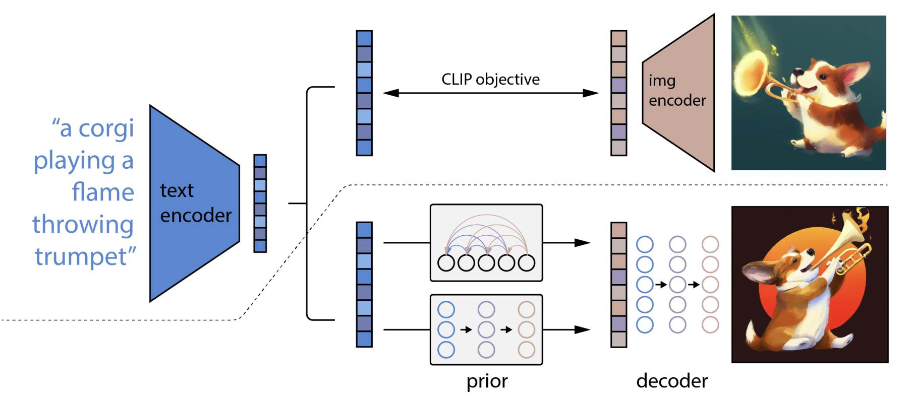
Dall-e 2
Text-to-image generators such as Dall-e, Midjourney, or Stable Diffusion combine LLM for text embedding with diffusion models for image generation.
CLIP embeddings of texts and images are first learned using contrastive learning.
A conditional diffusion process (GLIDE) then uses the image embeddings to produce images.
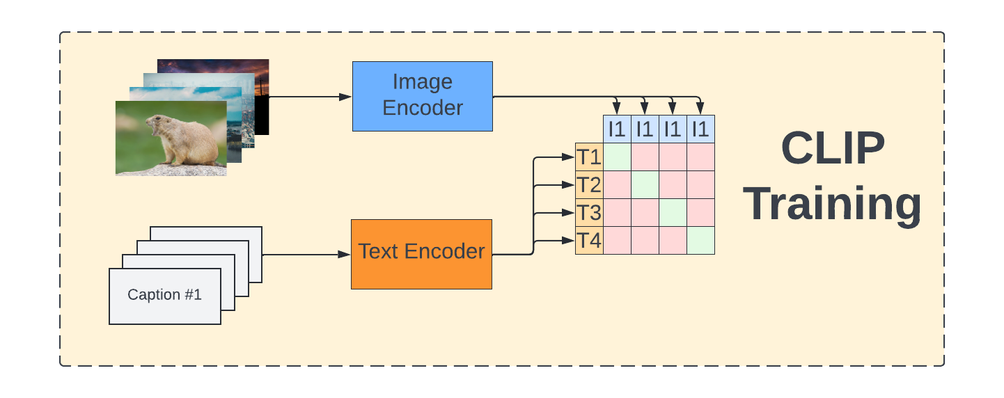
CLIP: Contrastive Language-Image Pre-training
Embeddings for text and images are learned using Transformer encoders and contrastive learning.
For each pair (text, image) in the training set, their representation should be made similar, while being different from the others.
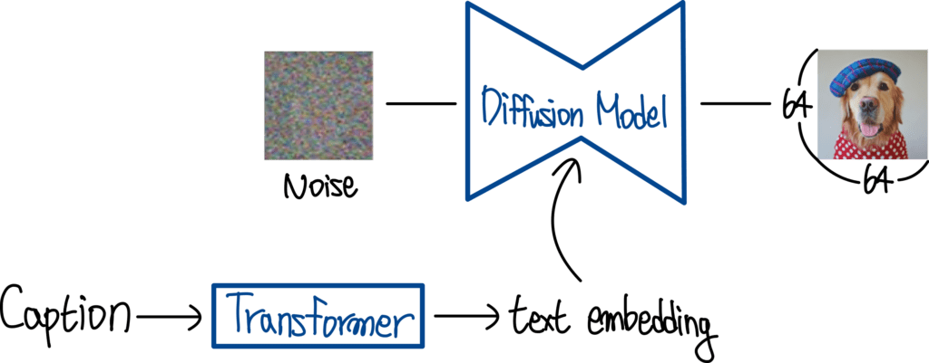
GLIDE
DDPMs generate images from raw noise, but there is no control over which image will emerge.
GLIDE (Guided Language to Image Diffusion for Generation and Editing) is a DDPM conditioned on a latent representation of a caption c.
As for cGAN and cVAE, the caption c is provided to the learned model:
\epsilon_\theta(x_t, t, c) \approx \epsilon_t
- Text embeddings can be obtained from any NLP model, for example a Transformer.
Dall-e 2
- In Dall-e 2, the prior network learns to map text embeddings to a sequence of image embeddings:
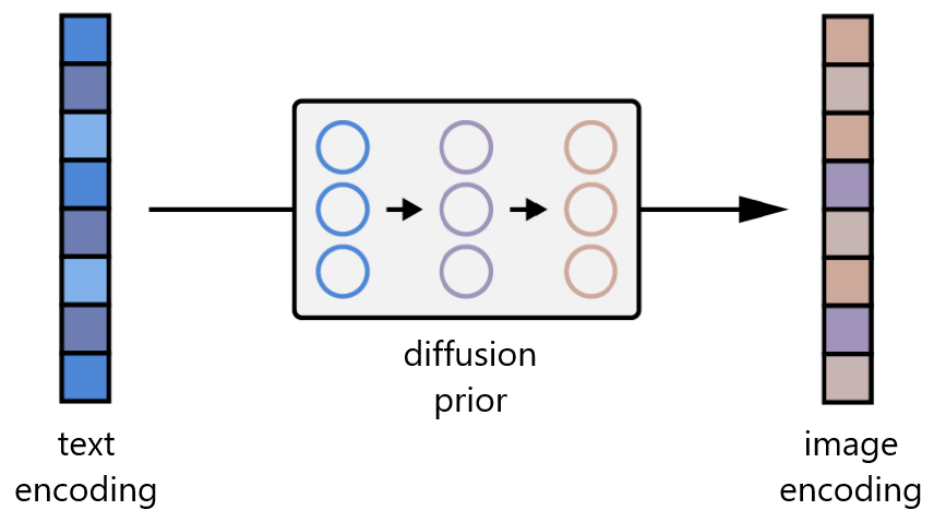
After CLIP training, the two embeddings are already close from each other, but the authors find that the diffusion process works better when the image embeddings change during the diffusion.
The image embedding is then used as the condition for GLIDE.