Neurocomputing
Autoencoders
Labeled vs unlabeled data
Supervised learning algorithms need a lot of labeled data (with \mathbf{t}) in order to learn classification/regression tasks, but labeled data is very expensive to obtain (experts, crowd sourcing).
A “bad” algorithm trained with a lot of data will perform better than a “good” algorithm trained with few data. “It is not who has the best algorithm who wins, it is who has the most data.”
Supervised learning
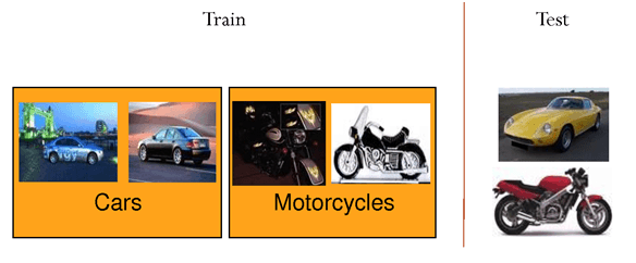
Self-taught learning
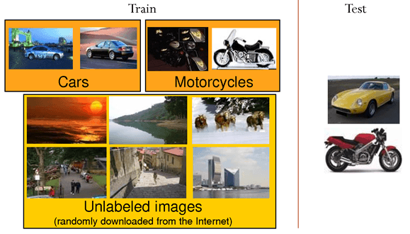
- Unlabeled data is only useful for unsupervised learning, but very cheap to obtain (camera, microphone, search engines). Can we combine efficiently both approaches? Self-taught learning or semi-supervised learning.
Autoencoders
- An autoencoder is a NN trying to learn the identity function f(\mathbf{x}) = \mathbf{x} using a different number of neurons in the hidden layer than in the input layer.
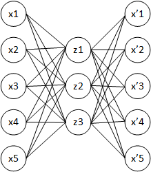
- An autoencoder minimizes the reconstruction loss between the input \mathbf{x} and the reconstruction \mathbf{x'}, for example the mse between the two vectors:
\mathcal{L}_\text{reconstruction}(\theta) = \mathbb{E}_{\mathbf{x} \in \mathcal{D}} [ ||\mathbf{x'} - \mathbf{x}||^2 ]
An autoencoder uses unsupervised learning: the output data used for learning is the same as the input data.
- No need for labels!
By forcing the projection of the input data on a feature space with less dimensions (latent space), the network has to extract relevant features from the training data.
- Dimensionality reduction, compression.
Result of training a sparse autoencoder on natural images
If the latent space has more dimensions than the input space, we need to constrain the autoencoder so that it does not simply learn the identity mapping.
Below is an example of a sparse autoencoder trained on natural images.
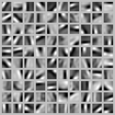
Inputs are taken from random natural images and cut in 10*10 patches.
100 features are extracted in the hidden layer.
The autoencoder is said sparse because it uses L1-regularization to make sure that only a few neurons are active in the hidden layer for a particular image.
The learned features look like what the first layer of a CNN would learn, except that there was no labels at all!
Can we take advantage of this to pre-train a supervised network?
Using an autoencoder for supervised learning

In supervised learning, deep neural networks suffer from many problems:
Local minima
Vanishing gradients
Long training times
All these problems are due to the fact that the weights are randomly initialized at the beginning of training.
Pretraining the weights using unsupervised learning allows to start already close to a good solution:
the network will need less steps to converge.
the gradients will vanish less.
less data is needed to learn a particular supervised task.
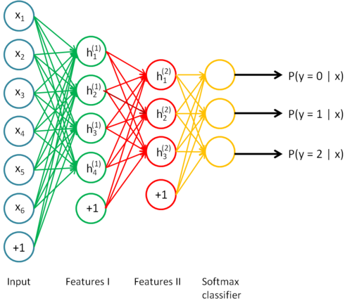
Stacked autoencoders
- Let’s try to learn a stacked autoencoder by learning progressively each feature vector.
http://ufldl.stanford.edu/wiki/index.php/Stacked_Autoencoders
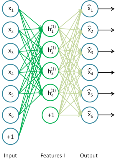
Stacked autoencoders
- Using unlabeled data, train an autoencoder to extract first-order features, freeze the weights and remove the decoder.
http://ufldl.stanford.edu/wiki/index.php/Stacked_Autoencoders
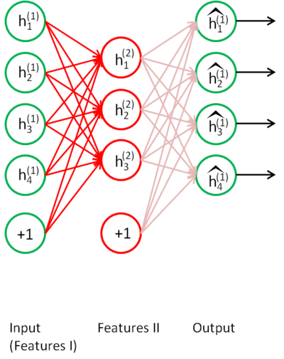
Stacked autoencoders
- Train another autoencoder on the same unlabeled data, but using the previous latent space as input/output.
http://ufldl.stanford.edu/wiki/index.php/Stacked_Autoencoders
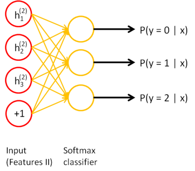
Stacked autoencoders
- Repeat the operation as often as needed, and finish with a simple classifier using the labeled data.
http://ufldl.stanford.edu/wiki/index.php/Stacked_Autoencoders
Greedy layer-wise learning
This defines a stacked autoencoder, trained using Greedy layer-wise learning.
Each layer progressively learns more and more complex features of the input data (edges - contour - forms - objects): feature extraction.
This method allows to train a deep network on few labeled data: the network will not overfit, because the weights are already in the right region.
It solves gradient vanishing, as the weights are already close to the optimal solution and will efficiently transmit the gradient backwards.
One can keep the pre-trained weights fixed for the classification task or fine-tune all the weights as in a regular DNN.
Application: Finding cats on the internet
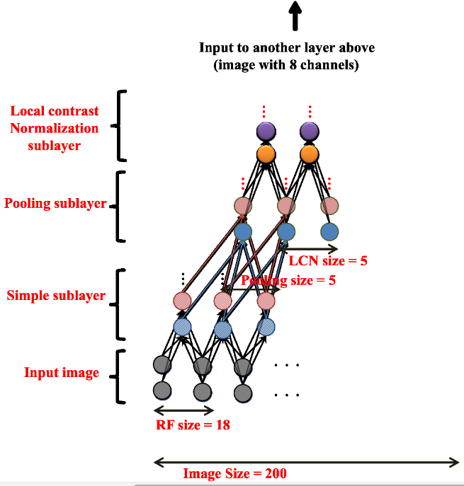
Andrew Ng and colleagues (Google, Stanford) used a similar technique to train a deep belief network on color images (200x200) taken from 10 million random unlabeled Youtube videos.
Each layer was trained greedily. They used a particular form of autoencoder called restricted Boltzmann machines (RBM) and a couple of other tricks (receptive fields, contrast normalization).
Training was distributed over 1000 machines (16.000 cores) and lasted for three days.
There was absolutely no task: the network just had to watch youtube videos.
After learning, they visualized what the neurons had learned.
Application: Finding cats on the internet
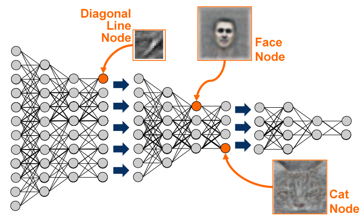

After training, some neurons had learned to respond uniquely to faces, or to cats, without ever having been instructed to.
The network can then be fine-tuned for classification tasks, improving the pre-AlexNet state-of-the-art on ImageNet by 70%.
Deep autoencoders
Autoencoders are not restricted to a single hidden layer.
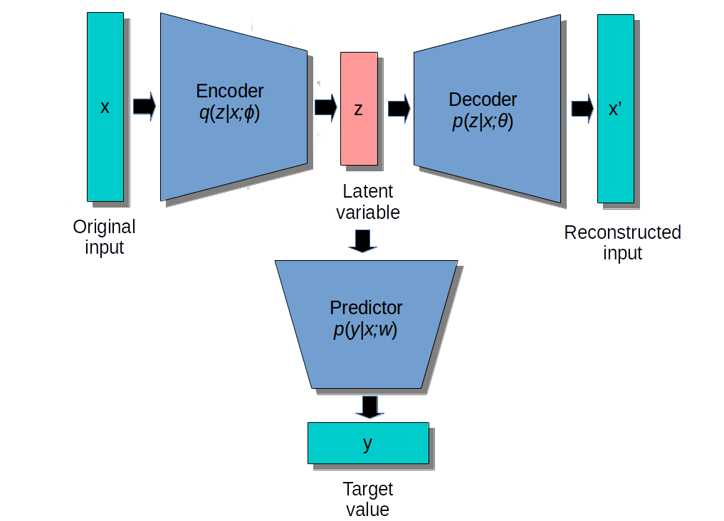
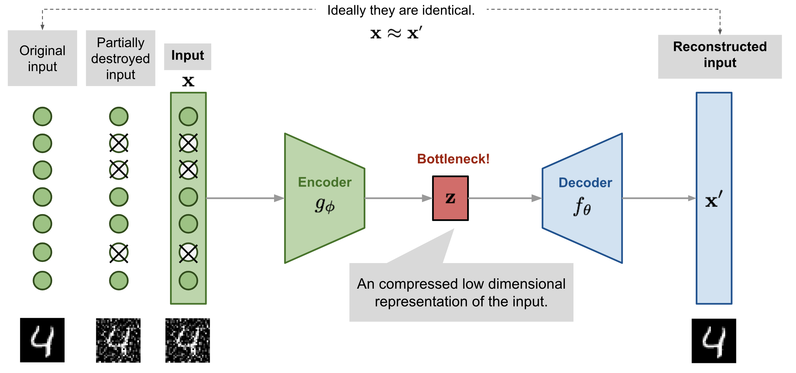
The encoder goes from the input space \mathbf{x} to the latent space \mathbf{z}.
\mathbf{z} = g_\phi(\mathbf{x})
- The decoder goes from the latent space \mathbf{z} to the output space \mathbf{x'}.
\mathbf{x'} = f_\theta(\mathbf{z})
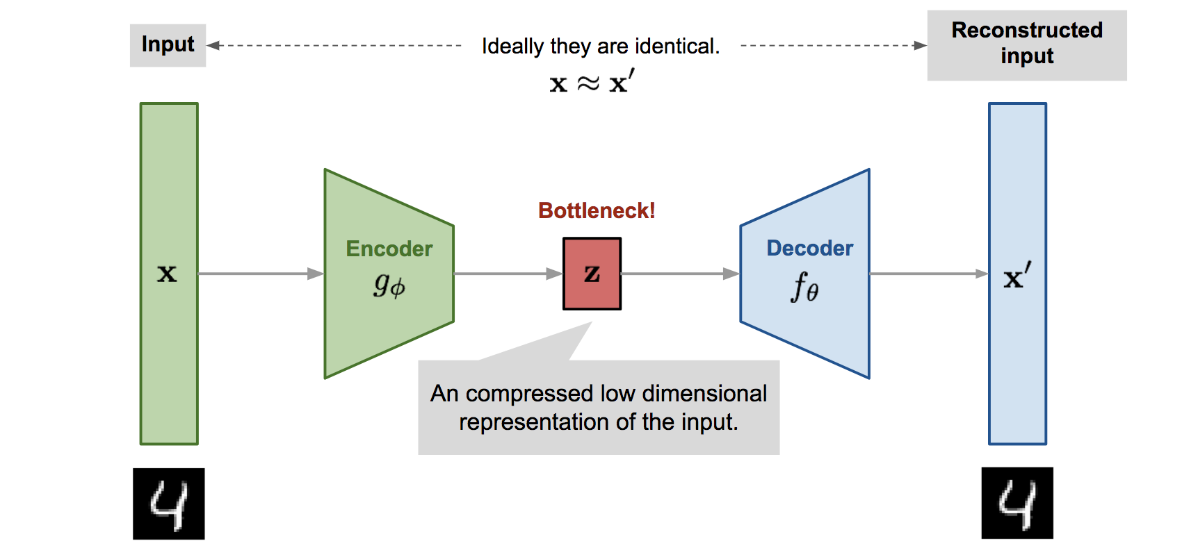
The latent space is a bottleneck layer of lower dimensionality, learning a compressed representation of the input which has to contain enough information in order to reconstruct the input.
Both the encoder with weights \phi and the decoder with weights \theta try to minimize the reconstruction loss:
\mathcal{L}_\text{reconstruction}(\theta, \phi) = \mathbb{E}_{\mathbf{x} \in \mathcal{D}} [ ||f_\theta(g_\phi(\mathbf{x})) - \mathbf{x}||^2 ]
- Learning is unsupervised: we only need input data.
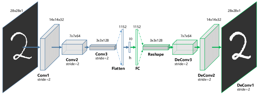
Deep autoencoders
The encoder and decoder can be anything: fully-connected, convolutional, recurrent, etc.
When using convolutional layers, the decoder has to upsample the latent space: max-unpooling or transposed convolutions can be used as in segmentation networks.
Semi-supervised learning
- In semi-supervised or self-taught learning, we can first train an autoencoder on huge amounts of unlabeled data, and then use the latent representations as an input to a shallow classifier on a small supervised dataset.
A linear classifier might even be enough if the latent space is well trained.
The weights of the encoder can be fine-tuned with backpropagation, or remain fixed.
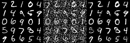
Denoising autoencoder
- A denoising autoencoder (DAE) is trained with noisy inputs (some pixels are dropped) but perfect desired outputs. It learns to suppress that noise.
Deep clustering
Clustering algorithms (k-means, Gaussian Mixture Models, spectral clustering, etc) can be applied in the latent space to group data points into clusters.
If you are lucky, the clusters may even correspond to classes.
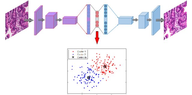
Source: doi:10.1007/978-3-030-32520-6_55
Motivation
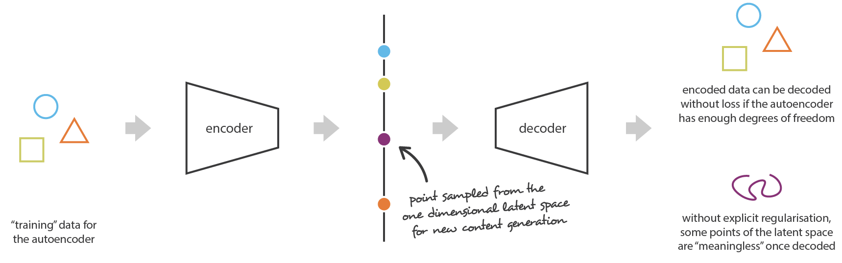
Autoencoders are deterministic: after learning, the same input \mathbf{x} will generate the same latent code \mathbf{z} and the same reconstruction \mathbf{\tilde{x}}.
Sampling the latent space generally generates non-sense reconstructions, because an autoencoder only learns data samples, it does not learn the underlying probability distribution.
Source: https://towardsdatascience.com/understanding-variational-autoencoders-vaes-f70510919f73
Data augmentation with autoencoders
The main problem of supervised learning is to get enough annotated data.
Being able to generate new images similar to the training examples would be extremely useful (data augmentation).
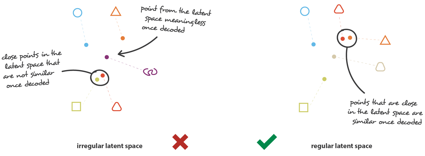
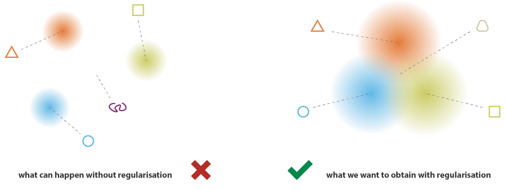
Regularized latent space
In order for this to work, we need to regularize the latent space:
- Close points in the latent space should correspond to close images.
“Classical” L1 or L2 regularization does not ensure the regularity of the latent space.
Source: https://towardsdatascience.com/understanding-variational-autoencoders-vaes-f70510919f73
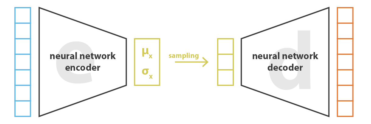
Variational autoencoder
The variational autoencoder (VAE) (Kingma and Ba, 2013) solves this problem by having the encoder represent the probability distribution q_\phi(\mathbf{z}|\mathbf{x}) instead of a point \mathbf{z} in the latent space.
This probability distribution is then sampled to obtain a vector \mathbf{z} that will be passed to the decoder p_\theta(\mathbf{z}).
The strong hypothesis is that the latent space follows a normal distribution with mean \mathbf{\mu_x} and variance \mathbf{\sigma_x}^2. \mathbf{z} \sim \mathcal{N}(\mathbf{\mu_x}, \mathbf{\sigma_x}^2)
The two vectors \mathbf{\mu_x} and \mathbf{\sigma_x}^2 are the outputs of the encoder.
Source: https://towardsdatascience.com/understanding-variational-autoencoders-vaes-f70510919f73
Sampling from a normal distribution

The normal distribution \mathcal{N}(\mu, \sigma^2) is fully defined by its two parameters:
\mu is the mean of the distribution.
\sigma^2 is its variance.
- The probability density function (pdf) of the normal distribution is defined by the Gaussian function:
f(x; \mu, \sigma) = \frac{1}{\sqrt{2\,\pi\,\sigma^2}} \, e^{-\displaystyle\frac{(x - \mu)^2}{2\,\sigma^2}}
A sample x will likely be close to \mu, with a deviation defined by \sigma^2.
It can be obtained using a sample of the standard normal distribution \mathcal{N}(0, 1):
x = \mu + \sigma \, \xi \; \; \text{with} \; \xi \sim \mathcal{N}(0, 1)
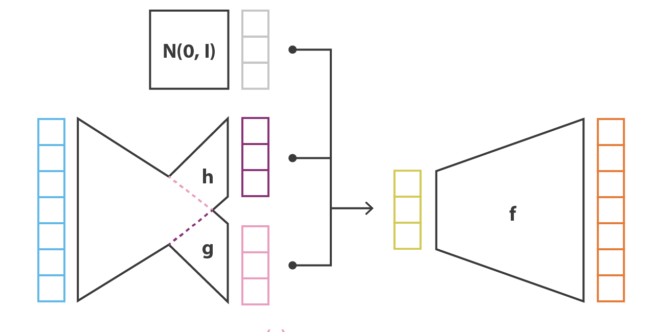
Variational autoencoder
Architecture of the VAE:
The encoder q_\phi(\mathbf{z}|\mathbf{x}) outputs the parameters \mathbf{\mu_x} and \mathbf{\sigma_x}^2 of a normal distribution \mathcal{N}(\mathbf{\mu_x}, \mathbf{\sigma_x}^2).
We sample one vector \mathbf{z} from this distribution: \mathbf{z} \sim \mathcal{N}(\mathbf{\mu_x}, \mathbf{\sigma_x}^2).
The decoder p_\theta(\mathbf{z}) reconstructs the input.
Open questions:
Which loss should we use and how do we regularize?
Does backpropagation still work?
Regularization term
Why do we want the latent distributions to be close from \mathcal{N}(\mathbf{0}, \mathbf{1}) for all inputs \mathbf{x}? \mathcal{L}(\theta, \phi) = \mathcal{L}_\text{reconstruction}(\theta, \phi) + \text{KL}(q_\phi(\mathbf{z}|\mathbf{x}) || \mathcal{N}(\mathbf{0}, \mathbf{1}))
By forcing the distributions to be close, we avoid “holes” in the latent space: we can move smoothly from one distribution to another without generating non-sense reconstructions.
Source: https://towardsdatascience.com/understanding-variational-autoencoders-vaes-f70510919f73
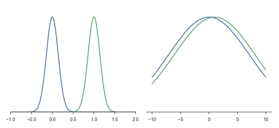
Why not regularize the mean and variance?
- To make q_\phi(\mathbf{z}|\mathbf{x}) close from \mathcal{N}(\mathbf{0}, \mathbf{1}), one could minimize the Euclidian distance in the parameter space:
\mathcal{L}(\theta, \phi) = \mathcal{L}_\text{reconstruction}(\theta, \phi) + (||\mathbf{\mu_x}||^2 + ||\mathbf{\sigma_x} - 1||^2)
However, this does not consider the overlap between the distributions.
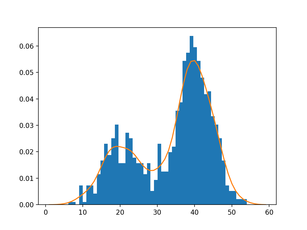
The two pairs of distributions below have the same distance between their means (0 and 1) and the same variance (1 and 10 respectively).
The distributions on the left are very different from each other, but the distance in the parameter space is the same.
Kullback-Leibler divergence
The KL divergence between two random distributions X and Y measures the statistical distance between them.
It describes, on average, how likely a sample from X could come from Y:
\text{KL}(X ||Y) = \mathbb{E}_{x \sim X}[- \log \frac{P(Y=x)}{P(X=x)}]

When the two distributions are equal almost anywhere, the KL divergence is 0. Otherwise it is positive.
Minimizing the KL divergence between two distributions makes them close in the statistical sense.
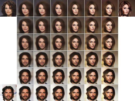
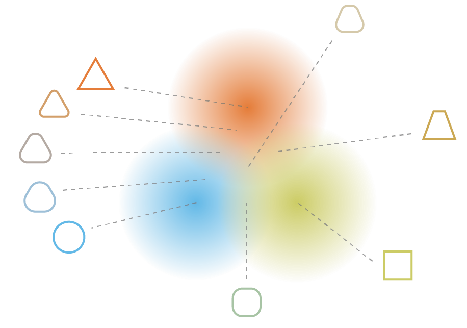
Regularization
Regularization tends to create a “gradient” over the information encoded in the latent space.
A point of the latent space sampled between the means of two encoded distributions should be decoded in an image in between the two training images.
Reparameterization trick
The second problem is that backpropagation does not work through the sampling operation.
It is easy to backpropagate the gradient of the loss function through the decoder until the sample \mathbf{z}.
But how do you backpropagate to the outputs of the encoder: \mathbf{\mu_x} and \mathbf{\sigma_x}?
- Modifying slightly \mathbf{\mu_x} or \mathbf{\sigma_x} may not change at all the sample \mathbf{z} \sim \mathcal{N}(\mathbf{\mu_x}, \mathbf{\sigma_x}^2), so you cannot estimate any gradient.
\frac{\partial \mathbf{z}}{\partial \mathbf{\mu_x}} = \; ?
Reparameterization trick
- Backpropagation does not work through a sampling operation, because it is not differentiable.
\mathbf{z} \sim \mathcal{N}(\mathbf{\mu_x}, \mathbf{\sigma_x}^2)
- The reparameterization trick consists in taking a sample \xi out of \mathcal{N}(0, 1) and reconstruct \mathbf{z} with:
\mathbf{z} = \mathbf{\mu_x} + \mathbf{\sigma_x} \, \xi \qquad \text{with} \qquad \xi \sim \mathcal{N}(0, 1)
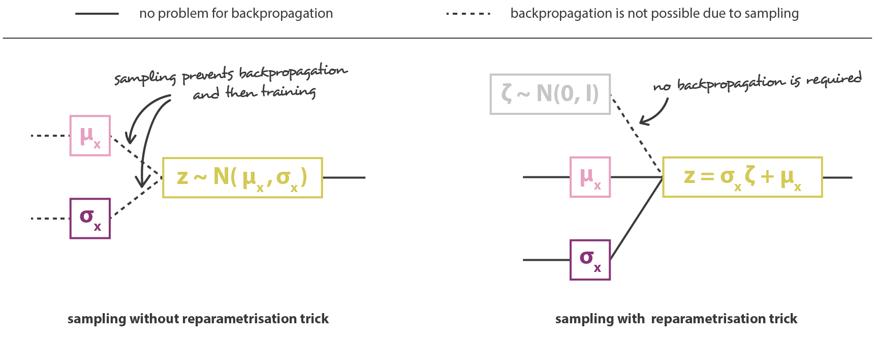
Source: https://towardsdatascience.com/understanding-variational-autoencoders-vaes-f70510919f73
Reparameterization trick
- The sampled value \xi \sim \mathcal{N}(0, 1) becomes just another input to the neural network.
Source: https://towardsdatascience.com/understanding-variational-autoencoders-vaes-f70510919f73
- It allows to transform \mathbf{\mu_x} and \mathbf{\sigma_x} into a sample \mathbf{z} of \mathcal{N}(\mathbf{\mu_x}, \mathbf{\sigma_x}^2):
\mathbf{z} = \mathbf{\mu_x} + \mathbf{\sigma_x} \, \xi
We do not need to backpropagate through \xi, as there is no parameter to learn!
The neural network becomes differentiable end-to-end, backpropagation will work.
Variational autoencoder
A variational autoencoder is an autoencoder where the latent space represents a probability distribution q_\phi(\mathbf{z} | \mathbf{x}) using the mean \mathbf{\mu_x} and standard deviation \mathbf{\sigma_x} of a normal distribution.
The latent space can be sampled to generate new images using the decoder p_\theta(\mathbf{z}).
KL regularization and the reparameterization trick are essential to VAE.

\begin{aligned} \mathcal{L}(\theta, \phi) &= \mathcal{L}_\text{reconstruction}(\theta, \phi) + \mathcal{L}_\text{regularization}(\phi) \\ &= \mathbb{E}_{\mathbf{x} \in \mathcal{D}, \xi \sim \mathcal{N}(0, 1)} [ - \log p_\theta(\mathbf{\mu_x} + \mathbf{\sigma_x} \, \xi) + \dfrac{1}{2} \, \sum_{k=1}^K (\mathbf{\sigma_x^2} + \mathbf{\mu_x}^2 -1 - \log \mathbf{\sigma_x^2})] \\ \end{aligned}
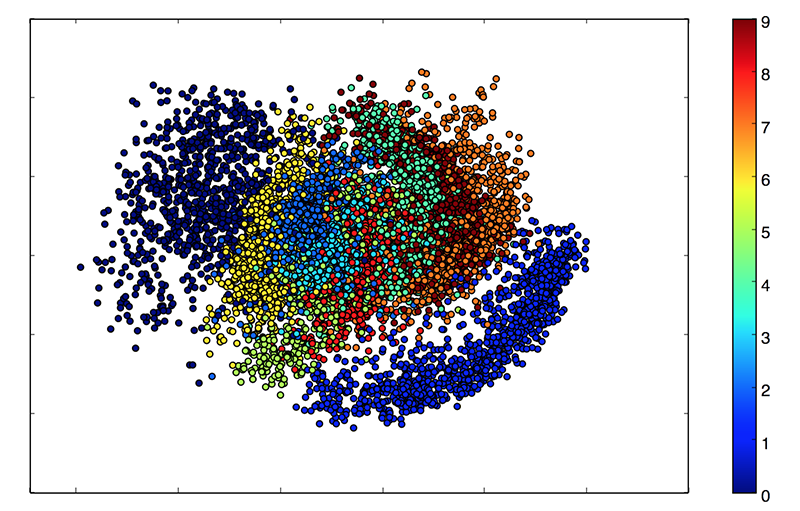
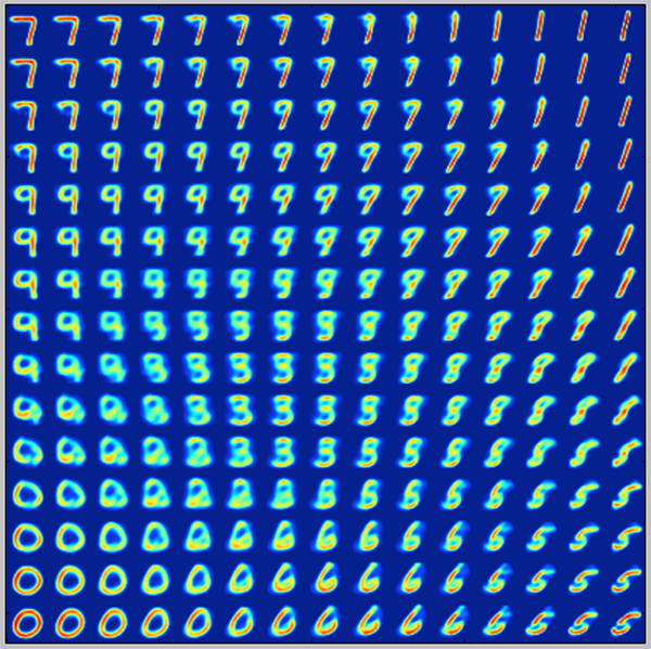
Variational autoencoder
- The two main applications of VAEs in unsupervised learning are:
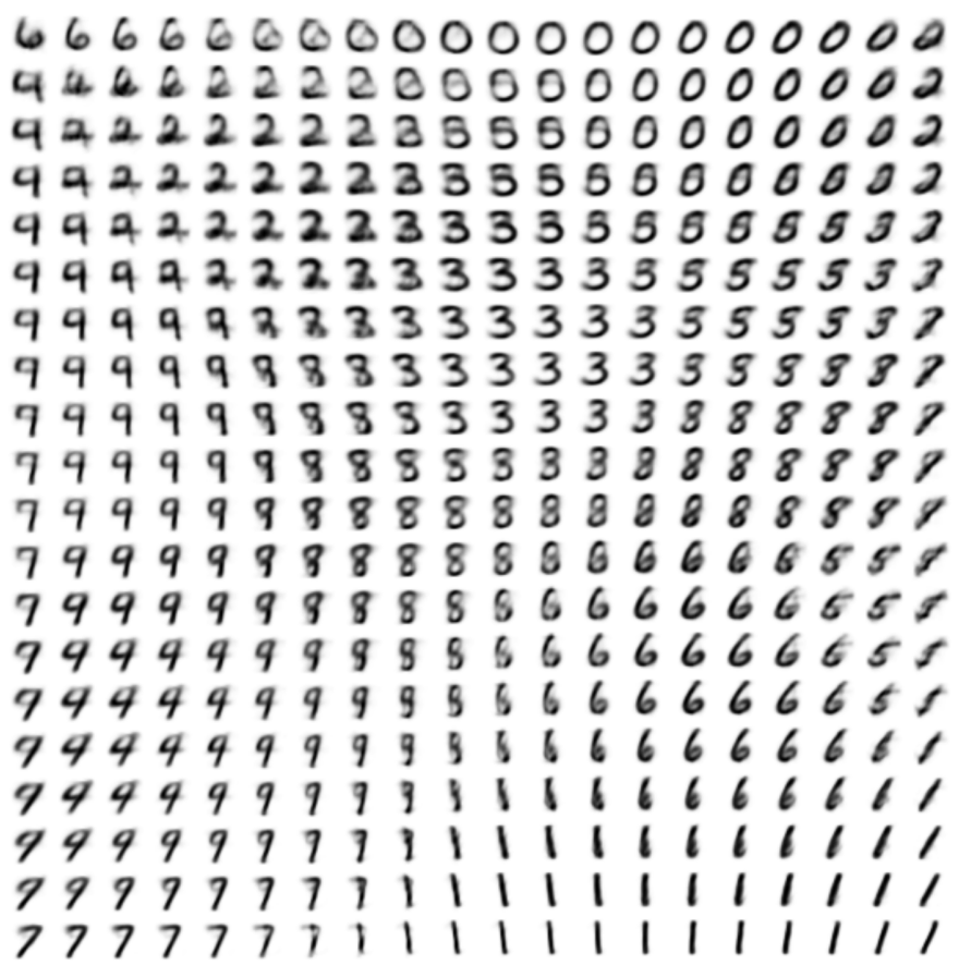
Dimensionality reduction: projecting high dimensional data (images) onto a smaller space, for example a 2D space for visualization.
Generative modeling: generating samples from the same distribution as the training data (data augmentation, deep fakes) by sampling on the manifold.
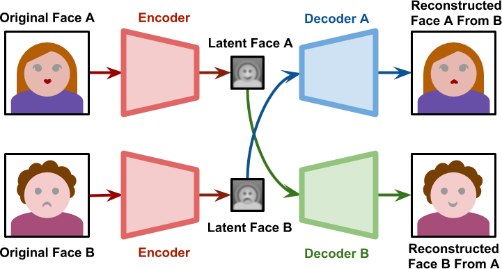
DeepFake
- During training, one encoder and two decoders learns to reproduce the face of each person.
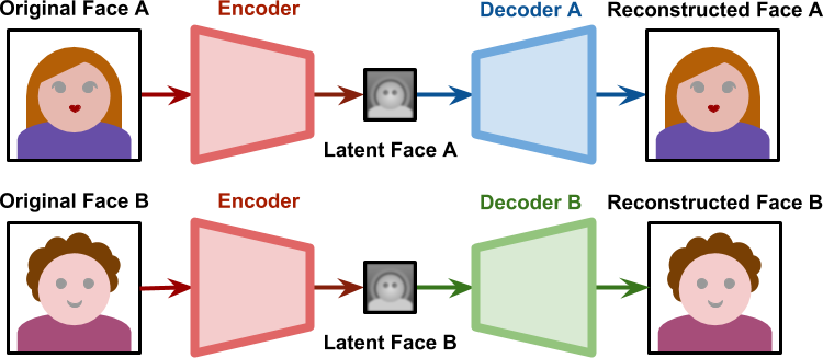
- When generating the deepfake, the decoder of person B is used on the latent representation of person A.
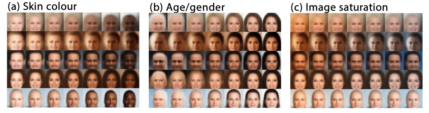
\beta-VAE
- VAE does not use a regularization parameter to balance the reconstruction and regularization losses. What happens if you do?
\begin{aligned} \mathcal{L}(\theta, \phi) &= \mathcal{L}_\text{reconstruction}(\theta, \phi) + \beta \, \mathcal{L}_\text{regularization}(\phi) \\ &= \mathbb{E}_{\mathbf{x} \in \mathcal{D}, \xi \sim \mathcal{N}(0, 1)} [ - \log p_\theta(\mathbf{\mu_x} + \mathbf{\sigma_x} \, \xi) + \dfrac{\beta}{2} \, \sum_{k=1}^K (\mathbf{\sigma_x^2} + \mathbf{\mu_x}^2 -1 - \log \mathbf{\sigma_x^2})] \\ \end{aligned}
Using \beta > 1 puts emphasis on learning statistically independent latent factors.
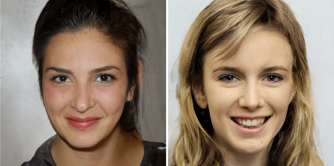
The \beta-VAE allows to disentangle the latent variables, i.e. manipulate them individually to vary only one aspect of the image (pose, color, gender, etc.).
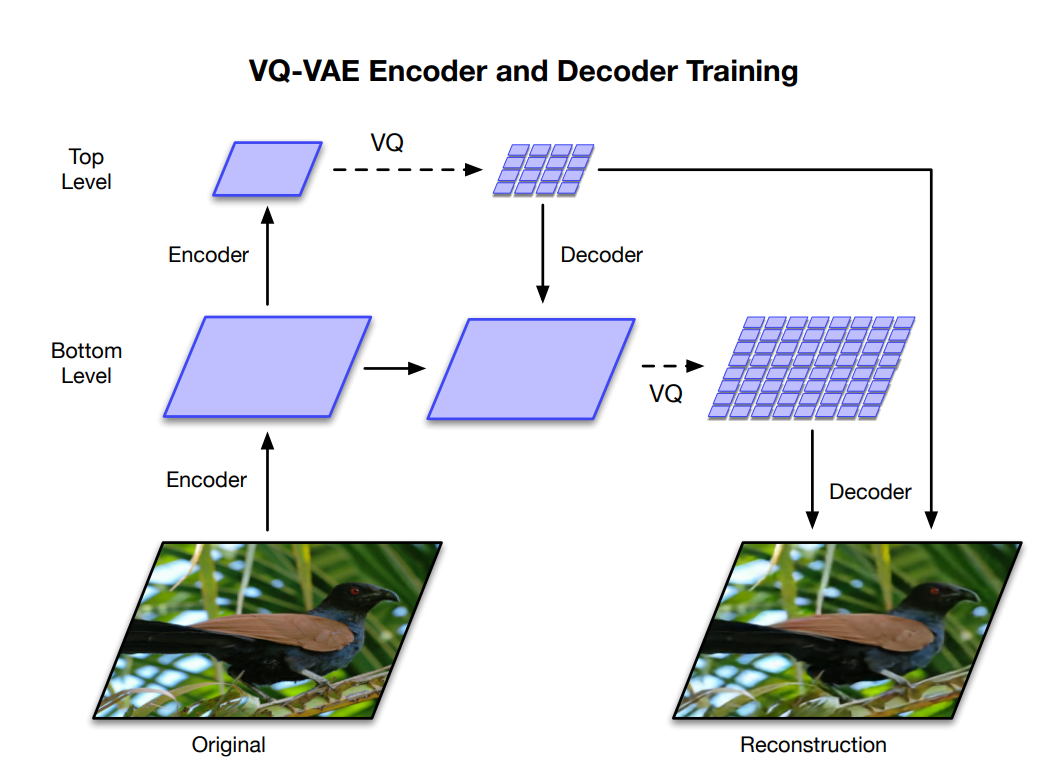
VQ-VAE
- Deepmind researchers proposed VQ-VAE-2, a hierarchical VAE using vector-quantized priors able to generate high-resolution images.
Conditional variational autoencoder (CVAE)
- What if we provide the labels to the encoder and the decoder during training?

Conditional variational autoencoder (CVAE)
- When trained with labels, the conditional variational autoencoder (CVAE) becomes able to sample many images of the same class.

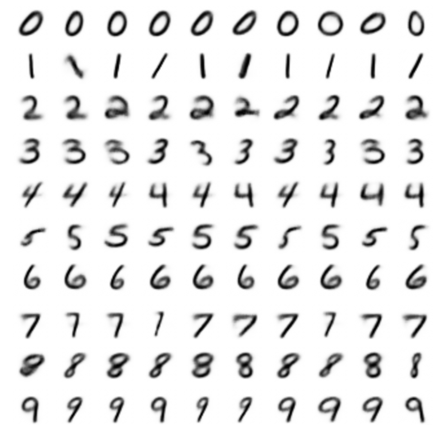
CVAE on MNIST
- CVAE allows to sample as many samples of a given class as we want: data augmentation.
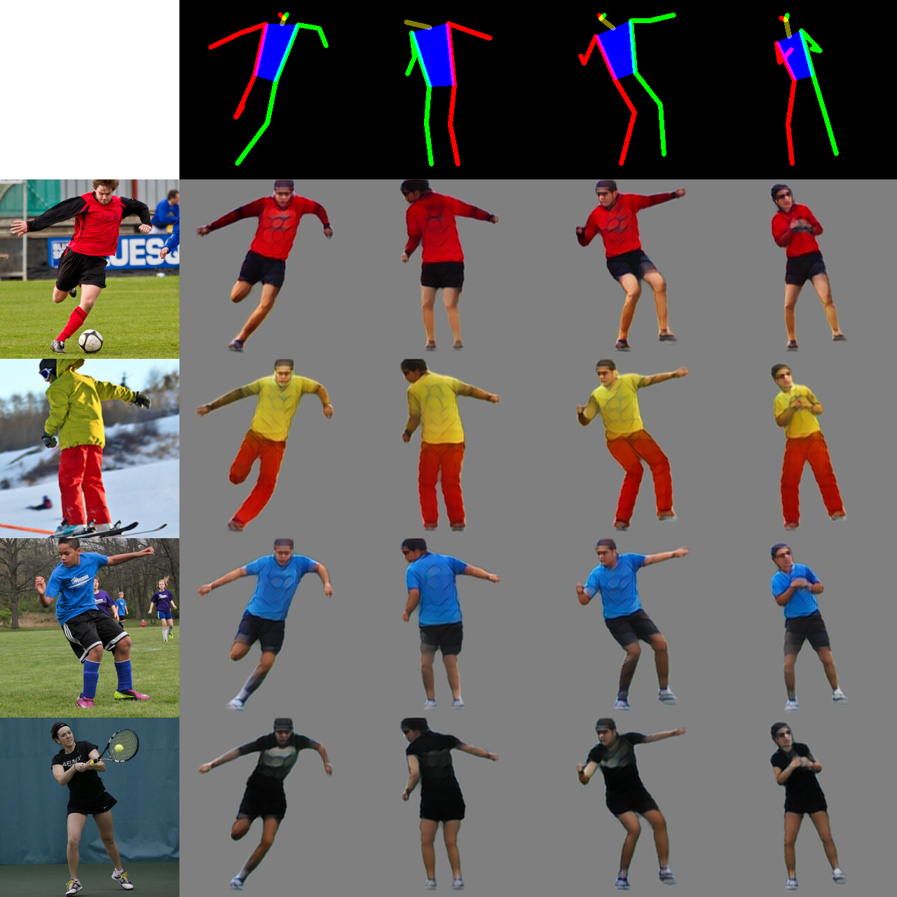
CVAE on shapes
- The condition does not need to be a label, it can be a shape or another image (passed through another encoder).
Learning probability distributions from samples
The input data X comes from an unknown distribution P(X). The training set \mathcal{D} is formed by samples of that distribution.
Learning the distribution of the data means learning a parameterized distribution p_\theta(X) that is as close as possible from the true distribution P(X).
The parameterized distribution could be a family of known distributions (e.g. normal) or a neural network with a softmax output layer.
- This means that we want to minimize the KL between the two distributions:
\min_\theta \, \text{KL}(P(X) || p_\theta(X)) = \mathbb{E}_{x \sim P(X)} [- \log \dfrac{p_\theta(X=x)}{P(X=x)}]
- The problem is that we do not know P(X) as it is what we want to learn, so we cannot estimate the KL directly.
Supervised learning
In supervised learning, we are learning the conditional probability P(T | X) of the targets given the inputs, i.e. what is the probability of having the label T=t given the input X=x.
A NN with a softmax output layer represents the parameterized distribution p_\theta(T | X).
The KL between the two distributions is:
\text{KL}(P(T | X) || p_\theta(T | X)) = \mathbb{E}_{x, t \sim \mathcal{D}} [- \log \dfrac{p_\theta(T=t | X=x)}{P(T=t | X=x)}]

- With the properties of the log, we know that the KL is the cross-entropy minus the entropy of the data:
\begin{aligned} \text{KL}(P(T | X) || p_\theta(T | X)) &= \mathbb{E}_{x, t \sim \mathcal{D}} [- \log p_\theta(T=t | X=x)] - \mathbb{E}_{x, t \sim \mathcal{D}} [- \log P(T=t | X=x)] \\ &\\ & = H(P(T | X), p_\theta(T |X)) - H(P(T|X)) \\ \end{aligned}
Curse of dimensionality
- The problem is that images are highly-dimensional (one dimension per pixel), so we would need astronomical numbers of samples to estimate the gradient (once): curse of dimensionality.
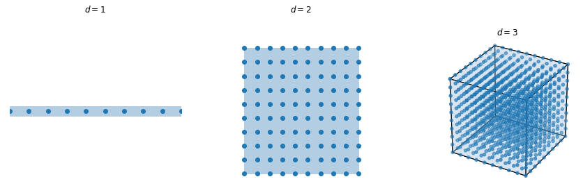
Source: https://dibyaghosh.com/blog/probability/highdimensionalgeometry.html
MLE does not work well in high-dimensional spaces.
We need to work in a much lower-dimensional space.
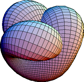
Manifolds
Images are not random samples of the pixel space: natural images are embedded in a much lower-dimensional space called a manifold.
A manifold is a locally Euclidian topological space of lower dimension.
The surface of the earth is locally flat and 2D, but globally spherical and 3D.
If we have a generative model telling us how a point on the manifold z maps to the image space (P(X | z)), we would only need to learn the distribution of the data in the lower-dimensional latent space.
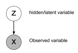
Generative model
The low-dimensional latent variables z are the actual cause for the observations X.
Given a sample z on the manifold, we can train a generative model p_\theta(X | z) to recreate the input X.
p_\theta(X | z) is the decoder: given a latent representation z, what is the corresponding observation X?
- If we learn the distribution p_\theta(z) of the manifold (latent space), we can infer the distribution of the data p_\theta(X) using that model:
p_\theta(X) = \mathbb{E}_{z \sim p_\theta(z)} [p_\theta(X | z)] = \int_z p_\theta(X | z) \, p_\theta(z) \, dz
- Problem: we do not know p_\theta(z), as the only data we see is X: z is called a latent variable because it explains the data but is hidden.
Variational inference
- The posterior is untractable as it would require to integrate over all possible inputs x \sim p_\theta(X):
p_\theta(z) = \mathbb{E}_{x \sim p_\theta(X)} [p_\theta(x |z) \, \dfrac{p_\theta(z)}{p_\theta(x)}] = \int_x p_\theta(x |z) \, p_\theta(z) \, dx
- Variational inference proposes to approximate the true encoder p_\theta(z | x) by another parameterized distribution q_\phi(z|x).
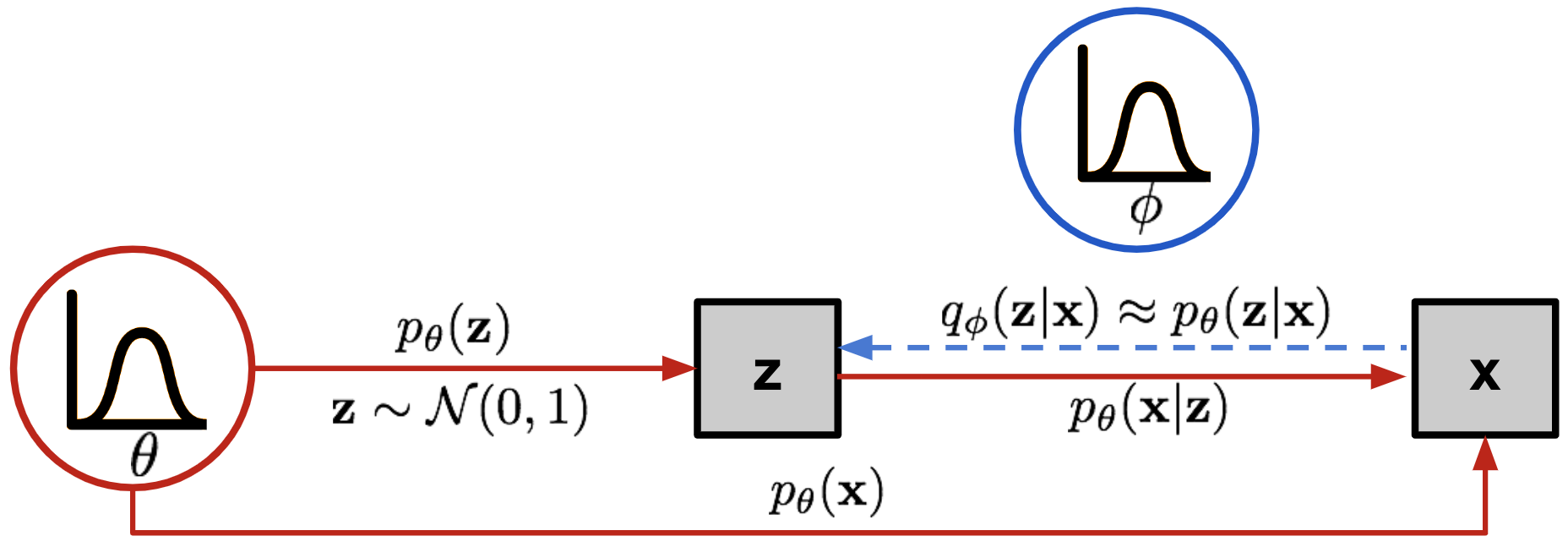
Source: https://lilianweng.github.io/lil-log/2018/08/12/from-autoencoder-to-beta-vae.html
The decoder p_\theta(x |z) generates observations x from a latent representation x with parameters \theta.
The encoder q_\phi(z|x) estimates the latent representation z of a generated observation x. It should approximate p_\theta(z | x) with parameters \phi.
Variational autoencoders
- Variational autoencoders use \mathcal{N}(0, 1) as a prior for the latent space, but any other prior could be used.
\begin{aligned} \mathcal{L}(\theta, \phi) &= \mathcal{L}_\text{reconstruction}(\theta, \phi) + \mathcal{L}_\text{regularization}(\phi) \\ &\\ &= \mathbb{E}_{\mathbf{x} \in \mathcal{D}, \mathbf{z} \sim q_\phi(\mathbf{z}|\mathbf{x})} [ - \log p_\theta(\mathbf{z})] + \text{KL}(q_\phi(\mathbf{z}|\mathbf{x}) || \mathcal{N}(\mathbf{0}, \mathbf{1}))\\ \end{aligned}
The reparameterization trick and the fact that the KL between normal distributions has a closed form allow us to use backpropagation end-to-end.
The encoder q_\phi(z|X) and decoder p_\theta(X | z) are neural networks in a VAE, but other parametrized distributions can be used (e.g. in physics).