Neurocomputing

Recurrent neural networks

Julien Vitay

Professur für Künstliche Intelligenz - Fakultät für Informatik

1 - RNN

Problem with feedforward networks

• Feedforward neural networks learn to associate an input vector to an output.

\mathbf{y} = F_\theta(\mathbf{x})

• If you present a sequence of inputs \mathbf{x}_0, \mathbf{x}_1, \ldots, \mathbf{x}_t to a feedforward network, the outputs will be independent from each other:

\mathbf{y}_0 = F_\theta(\mathbf{x}_0) \mathbf{y}_1 = F_\theta(\mathbf{x}_1) \dots \mathbf{y}_t = F_\theta(\mathbf{x}_t)

• Many problems depend on time series, such as predicting the future of a time series by knowing its past values.

x_{t+1} = F_\theta(x_0, x_1, \ldots, x_t)

• Example: weather forecast, financial prediction, predictive maintenance, video analysis…

Input aggregation

• A naive solution is to aggregate (concatenate) inputs over a sufficiently long window and use it as a new input vector for the feedforward network.

\mathbf{X} = \begin{bmatrix}\mathbf{x}_{t-T} & \mathbf{x}_{t-T+1} & \ldots & \mathbf{x}_t \\ \end{bmatrix}

\mathbf{y}_t = F_\theta(\mathbf{X})

https://www.researchgate.net/publication/220827486_A_study_on_the_ability_of_Support_Vector_Regression_and_Neural_Networks_to_Forecast_Basic_Time_Series_Patterns

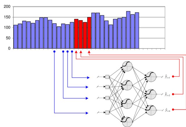
• Problem 1: How long should the window be?

• Problem 2: Having more input dimensions increases dramatically the complexity of the classifier (VC dimension), hence the number of training examples required to avoid overfitting.

Recurrent neural network

Source: http://colah.github.io/posts/2015-08-Understanding-LSTMs

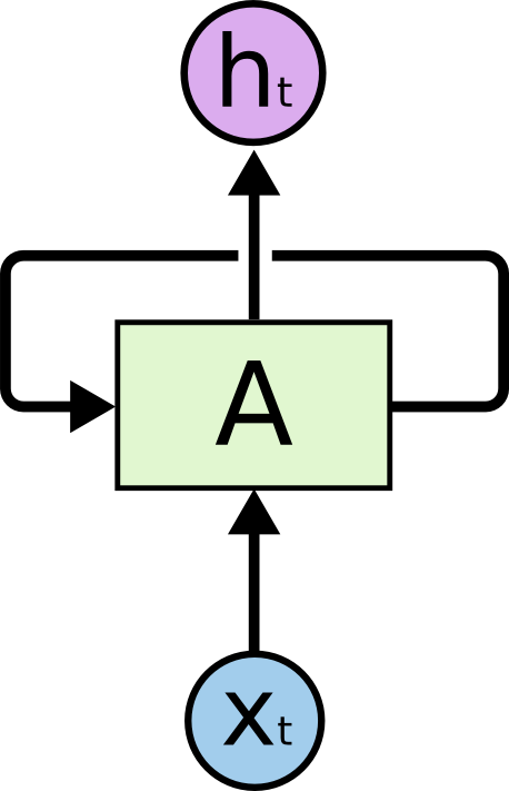
• A recurrent neural network (RNN) uses it previous output as an additional input (context).

• All vectors have a time index t denoting the time at which this vector was computed.

• The input vector at time t is \mathbf{x}_t, the output vector is \mathbf{h}_t:

\mathbf{h}_t = \sigma(W_x \times \mathbf{x}_t + W_h \times \mathbf{h}_{t-1} + \mathbf{b})

• \sigma is a transfer function, usually logistic or tanh.

• The input \mathbf{x}_t and previous output \mathbf{h}_{t-1} are multiplied by learnable weights:

  • W_x is the input weight matrix.

  • W_h is the recurrent weight matrix.

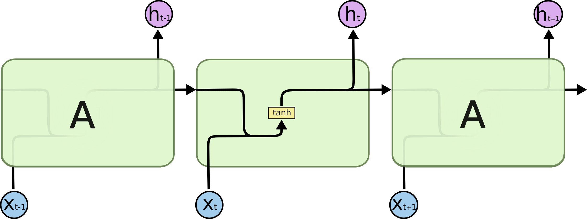
Recurrent neural networks

Source: http://colah.github.io/posts/2015-08-Understanding-LSTMs

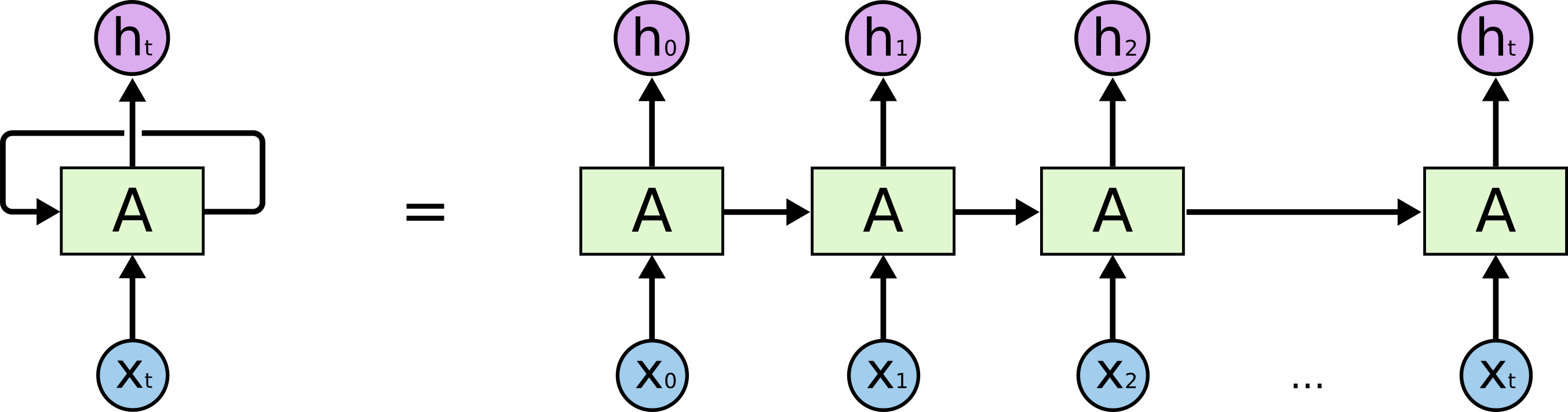
• One can unroll a recurrent network: the output \mathbf{h}_t depends on the whole history of inputs from \mathbf{x}_0 to \mathbf{x}_t.

\begin{aligned} \mathbf{h}_t & = \sigma(W_x \times \mathbf{x}_t + W_h \times \mathbf{h}_{t-1} + \mathbf{b}) \\ & = \sigma(W_x \times \mathbf{x}_t + W_h \times \sigma(W_x \times \mathbf{x}_{t-1} + W_h \times \mathbf{h}_{t-2} + \mathbf{b}) + \mathbf{b}) \\ & = f_{W_x, W_h, \mathbf{b}} (\mathbf{x}_0, \mathbf{x}_1, \dots,\mathbf{x}_t) \\ \end{aligned}

• A RNN is considered as part of deep learning, as there are many layers of weights between the first input \mathbf{x}_0 and the output \mathbf{h}_t.

• The only difference with a DNN is that the weights W_x and W_h are reused at each time step.

BPTT: Backpropagation through time

Source: http://colah.github.io/posts/2015-08-Understanding-LSTMs

\mathbf{h}_t = f_{W_x, W_h, \mathbf{b}} (\mathbf{x}_0, \mathbf{x}_1, \dots,\mathbf{x}_t) \\

• The function between the history of inputs and the output at time t is differentiable: we can simply apply gradient descent to find the weights!

• This variant of backpropagation is called Backpropagation Through Time (BPTT).

• Once the loss between \mathbf{h}_t and its desired value is computed, one applies the chain rule to find out how to modify the weights W_x and W_h using the history (\mathbf{x}_0, \mathbf{x}_1, \ldots, \mathbf{x}_t).

BPTT: Backpropagation through time

• Let’s compute the gradient accumulated between \mathbf{h}_{t-1} and \mathbf{h}_{t}:

\begin{aligned} \mathbf{h}_{t} & = \sigma(W_x \times \mathbf{x}_{t} + W_h \times \mathbf{h}_{t-1} + \mathbf{b}) \\ \end{aligned}

• As for feedforward networks, the gradient of the loss function is decomposed into two parts:

\frac{\partial \mathcal{L}(W_x, W_h)}{\partial W_x} = \frac{\partial \mathcal{L}(W_x, W_h)}{\partial \mathbf{h}_t} \times \frac{\partial \mathbf{h}_t}{\partial W_x}

\frac{\partial \mathcal{L}(W_x, W_h)}{\partial W_h} = \frac{\partial \mathcal{L}(W_x, W_h)}{\partial \mathbf{h}_t} \times \frac{\partial \mathbf{h}_t}{\partial W_h}

• The first part only depends on the loss function (mse, cross-entropy):

\frac{\partial \mathcal{L}(W_x, W_h)}{\partial \mathbf{h}_t} = - (\mathbf{t}_{t}- \mathbf{h}_{t})

• The second part depends on the RNN itself.

BPTT: Backpropagation through time

• Output of the RNN:

\begin{aligned} \mathbf{h}_{t} & = \sigma(W_x \times \mathbf{x}_{t} + W_h \times \mathbf{h}_{t-1} + \mathbf{b}) \\ \end{aligned}

• The gradients w.r.t the two weight matrices are given by this recursive relationship (product rule):

\begin{aligned} \frac{\partial \mathbf{h}_t}{\partial W_x} & = \mathbf{h'}_{t} \times (\mathbf{x}_t + W_h \times \frac{\partial \mathbf{h}_{t-1}}{\partial W_x})\\ & \\ \frac{\partial \mathbf{h}_t}{\partial W_h} & = \mathbf{h'}_{t} \times (\mathbf{h}_{t-1} + W_h \times \frac{\partial \mathbf{h}_{t-1}}{\partial W_h})\\ \end{aligned}

• The derivative of the transfer function is noted \mathbf{h'}_{t}:

\mathbf{h'}_{t} = \begin{cases} \mathbf{h}_{t} \, (1 - \mathbf{h}_{t}) \quad \text{ for logistic}\\ (1 - \mathbf{h}_{t}^2) \quad \text{ for tanh.}\\ \end{cases}

BPTT: Backpropagation through time

• If we unroll the gradient, we obtain:

\begin{aligned} \frac{\partial \mathbf{h}_t}{\partial W_x} & = \mathbf{h'}_{t} \, (\mathbf{x}_t + W_h \times \mathbf{h'}_{t-1} \, (\mathbf{x}_{t-1} + W_h \times \mathbf{h'}_{t-2} \, (\mathbf{x}_{t-2} + W_h \times \ldots (\mathbf{x}_0))))\\ & \\ \frac{\partial \mathbf{h}_t}{\partial W_h} & = \mathbf{h'}_{t} \, (\mathbf{h}_{t-1} + W_h \times \mathbf{h'}_{t-1} \, (\mathbf{h}_{t-2} + W_h \times \mathbf{h'}_{t-2} \, \ldots (\mathbf{h}_{0})))\\ \end{aligned}

• When updating the weights at time t, we need to store in memory:

  • the complete history of inputs \mathbf{x}_0, \mathbf{x}_1, … \mathbf{x}_t.

  • the complete history of outputs \mathbf{h}_0, \mathbf{h}_1, … \mathbf{h}_t.

  • the complete history of derivatives \mathbf{h'}_0, \mathbf{h'}_1, … \mathbf{h'}_t.

before computing the gradients iteratively, starting from time t and accumulating gradients backwards in time until t=0.

• Each step backwards in time adds a bit to the gradient used to update the weights.

Truncated BPTT

Source: https://r2rt.com/styles-of-truncated-backpropagation.html

• In practice, going back to t=0 at each time step requires too many computations, which may not be needed.

• Truncated BPTT only updates the gradients up to T steps before: the gradients are computed backwards from t to t-T. The partial derivative in t-T-1 is considered 0.

• This limits the horizon of BPTT: dependencies longer than T will not be learned, so it has to be chosen carefully for the task.

• T becomes yet another hyperparameter of your algorithm…

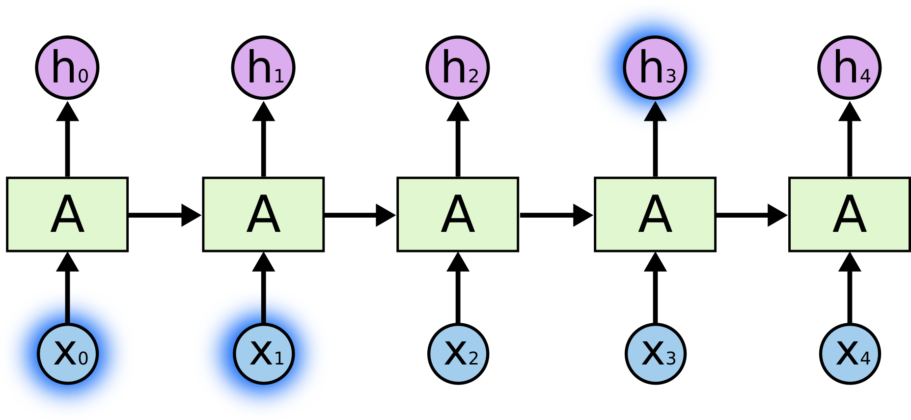
Temporal dependencies

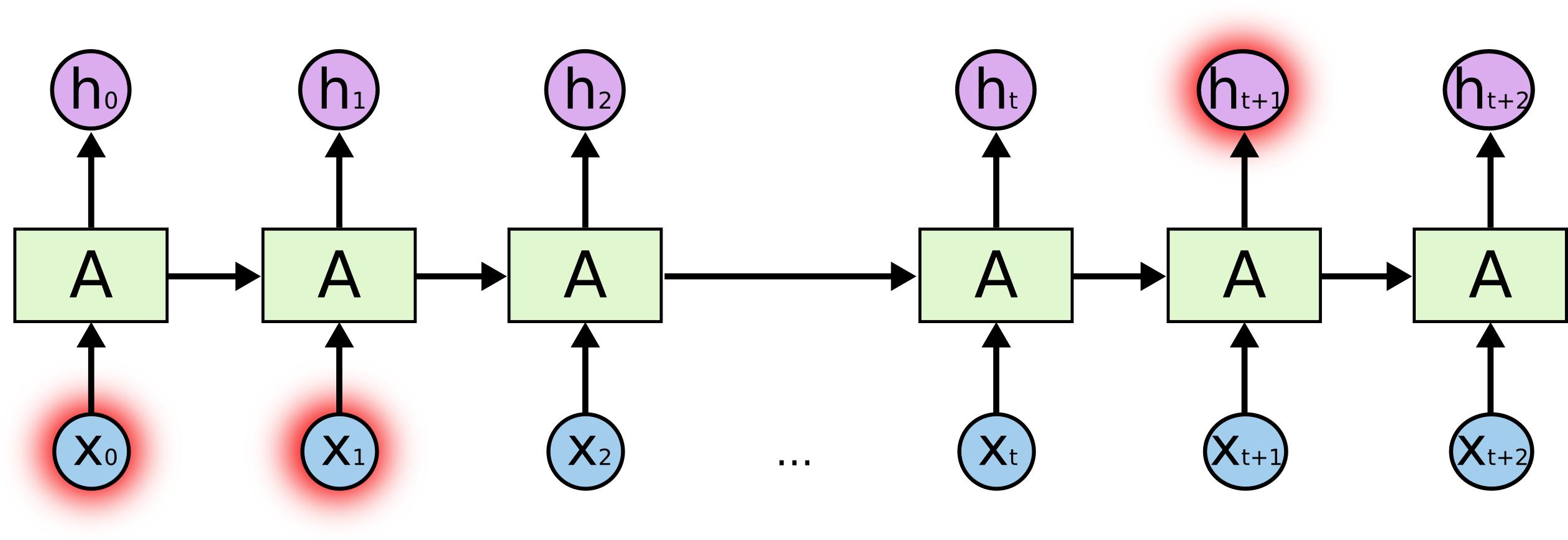
• BPTT is able to find short-term dependencies between inputs and outputs: perceiving the inputs \mathbf{x}_0 and \mathbf{x}_1 allows to respond correctly at t = 3.

Source: http://colah.github.io/posts/2015-08-Understanding-LSTMs

Temporal dependencies

• But it fails to detect long-term dependencies because of:

  • the truncated horizon T (for computational reasons).

  • the vanishing gradient problem.

Source: http://colah.github.io/posts/2015-08-Understanding-LSTMs

Vanishing and exploding gradients

• Let’s look at the gradient w.r.t to the input weights:

\begin{aligned} \frac{\partial \mathbf{h}_t}{\partial W_x} & = \mathbf{h'}_{t} \, (\mathbf{x}_t + W_h \times \frac{\partial \mathbf{h}_{t-1}}{\partial W_x})\\ & \\ \end{aligned}

• At each iteration backwards in time, the gradients are multiplied by W_h.

• If you search how \frac{\partial \mathbf{h}_t}{\partial W_x} depends on \mathbf{x}_0, you obtain something like:

\begin{aligned} \frac{\partial \mathbf{h}_t}{\partial W_x} & \approx \prod_{k=0}^t \mathbf{h'}_{k} \, ((W_h)^t \, \mathbf{x}_0 + \dots) \\ \end{aligned}

• If |W_h| > 1, |(W_h)^t| increases exponentially with t: the gradient explodes.

• If |W_h| < 1, |(W_h)^t| decreases exponentially with t: the gradient vanishes.

Vanishing and exploding gradients

• Exploding gradients are relatively easy to deal with: one just clips the norm of the gradient to a maximal value.

|| \frac{\partial \mathcal{L}(W_x, W_h)}{\partial W_x}|| \gets \min(||\frac{\partial \mathcal{L}(W_x, W_h)}{\partial W_x}||, T)

• But there is no solution to the vanishing gradient problem for regular RNNs: the gradient fades over time (backwards) and no long-term dependency can be learned.

• This is the same problem as for feedforward deep networks: a RNN is just a deep network rolled over itself.

• Its depth (number of layers) corresponds to the maximal number of steps back in time.

• In order to limit vanishing gradients and learn long-term dependencies, one has to use a more complex structure for the layer.

• This is the idea behind long short-term memory (LSTM) networks.

2 - LSTM

Regular RNN

Source: http://colah.github.io/posts/2015-08-Understanding-LSTMs

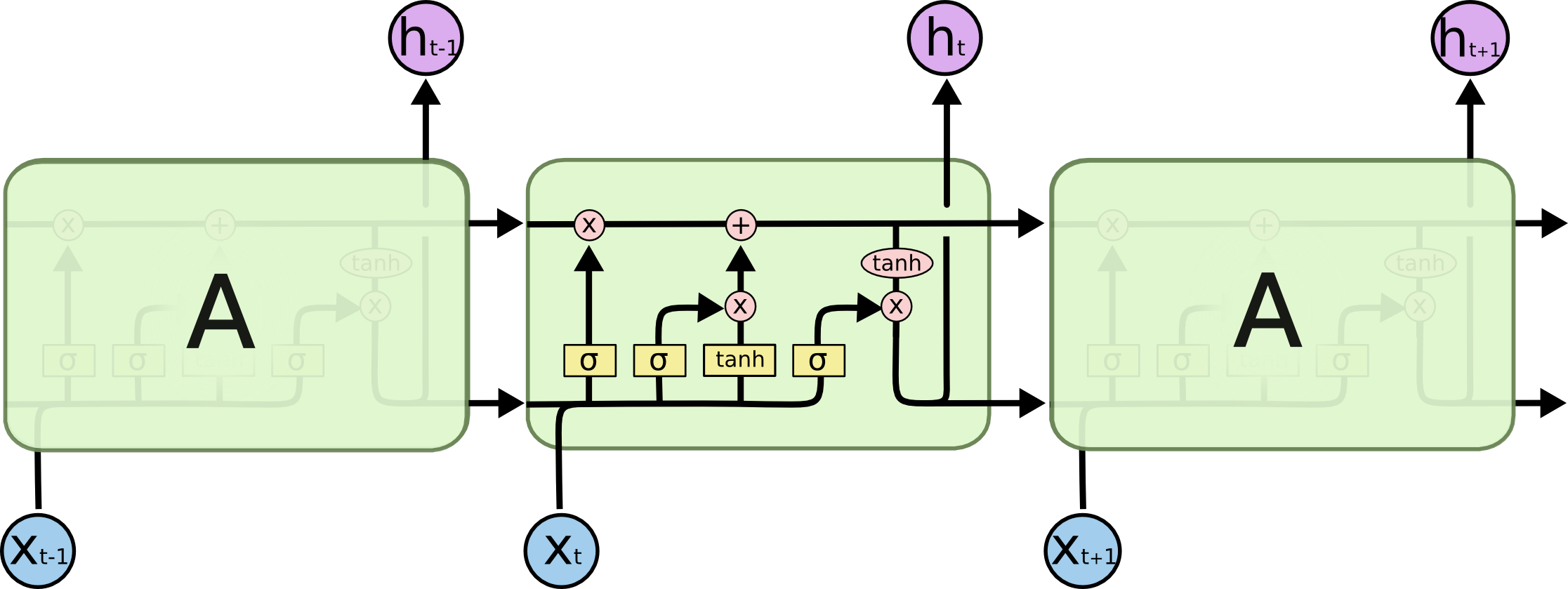
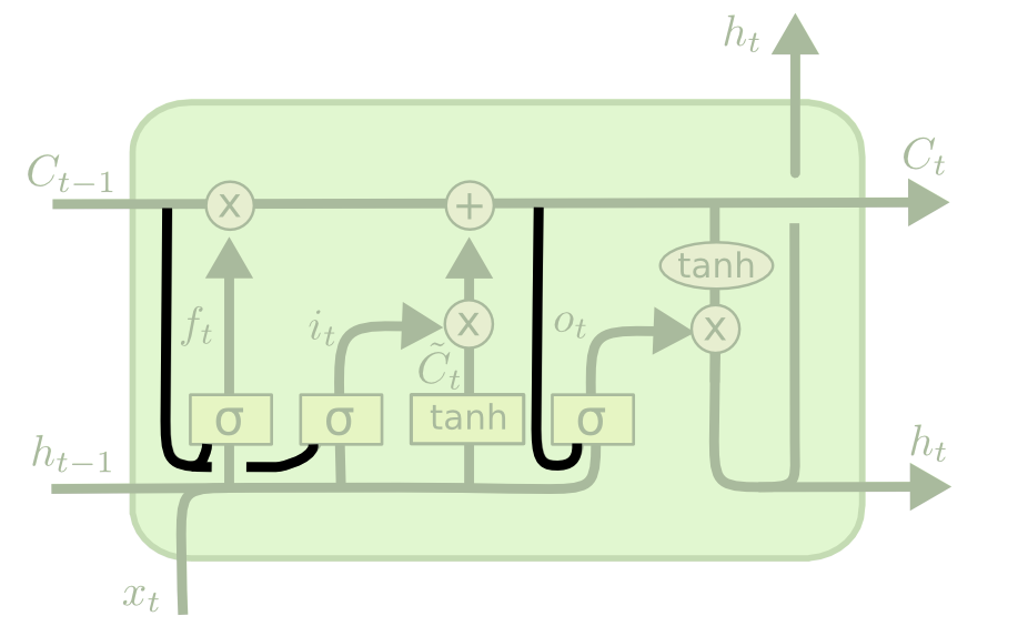
LSTM

Source: http://colah.github.io/posts/2015-08-Understanding-LSTMs

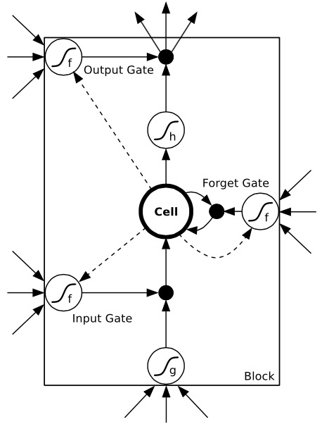
LSTM cell

Source: http://colah.github.io/posts/2015-08-Understanding-LSTMs

• A LSTM layer is a RNN layer with the ability to control what it memorizes.

• In addition to the input \mathbf{x}_t and output \mathbf{h}_t, it also has a state \mathbf{C}_t which is maintained over time.

• The state is the memory of the layer (sometimes called context).

• It also contains three multiplicative gates:

  • The input gate controls which inputs should enter the memory.

  • The forget gate controls which memory should be forgotten.

  • The output gate controls which part of the memory should be used to produce the output.

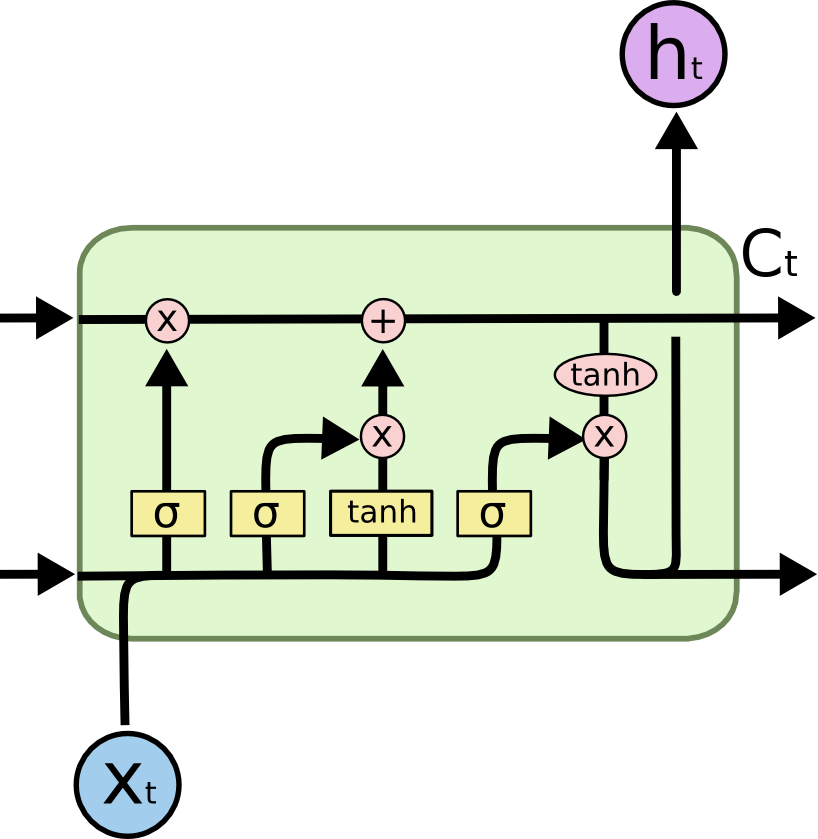
LSTM cell

Source: http://eric-yuan.me/rnn2-lstm/

• The state \mathbf{C}_t can be seen as an accumulator integrating inputs (and previous outputs) over time.

  • The input gate allows inputs to be stored.

    • are they worth remembering?

  • The forget gate “empties” the accumulator

    • do I still need them?

  • The output gate allows to use the accumulator for the output.

    • should I respond now? Do I have enough information?

• The gates learn to open and close through learnable weights.

The cell state is propagated over time

Source: http://colah.github.io/posts/2015-08-Understanding-LSTMs

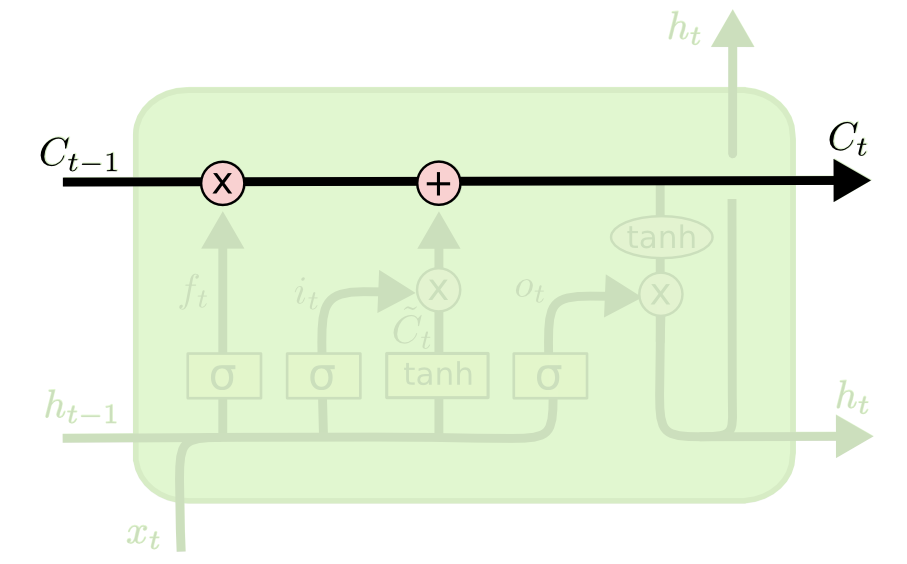
• By default, the cell state \mathbf{C}_t stays the same over time (conveyor belt).

• It can have the same number of dimensions as the output \mathbf{h}_t, but does not have to.

• Its content can be erased by multiplying it with a vector of 0s, or preserved by multiplying it by a vector of 1s.

• We can use a sigmoid to achieve this:

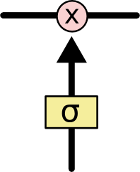
The forget gate

Source: http://colah.github.io/posts/2015-08-Understanding-LSTMs

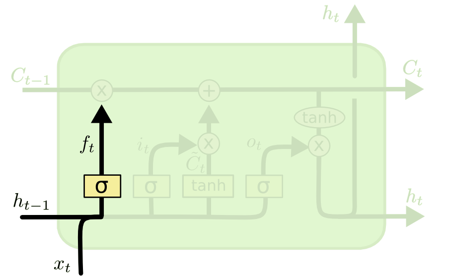
• Forget weights W_f and a sigmoid function are used to decide if the state should be preserved or not.

\mathbf{f}_t = \sigma(W_f \times [\mathbf{h}_{t-1}; \mathbf{x}_t] + \mathbf{b}_f)

• [\mathbf{h}_{t-1}; \mathbf{x}_t] is simply the concatenation of the two vectors \mathbf{h}_{t-1} and \mathbf{x}_t.

• \mathbf{f}_t is a vector of values between 0 and 1, one per dimension of the cell state \mathbf{C}_t.

The input gate

Source: http://colah.github.io/posts/2015-08-Understanding-LSTMs

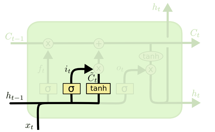
• Similarly, the input gate uses a sigmoid function to decide if the state should be updated or not.

\mathbf{i}_t = \sigma(W_i \times [\mathbf{h}_{t-1}; \mathbf{x}_t] + \mathbf{b}_i)

• As for RNNs, the input \mathbf{x}_t and previous output \mathbf{h}_{t-1} are combined to produce a candidate state \tilde{\mathbf{C}}_t using the tanh transfer function.

\tilde{\mathbf{C}}_t = \text{tanh}(W_C \times [\mathbf{h}_{t-1}; \mathbf{x}_t] + \mathbf{b}_c)

Updating the state

Source: http://colah.github.io/posts/2015-08-Understanding-LSTMs

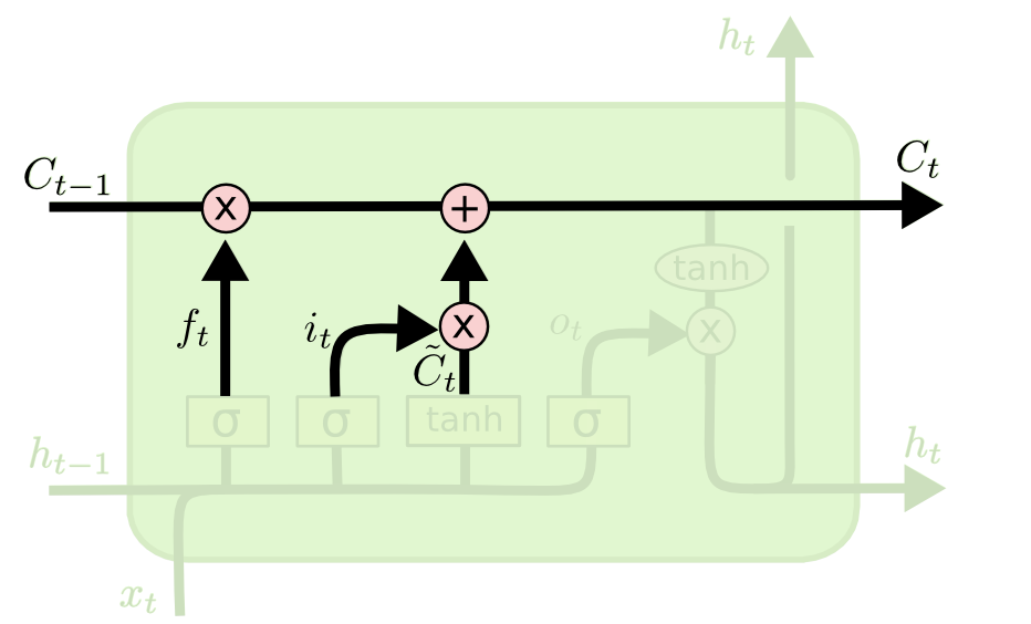
• The new state \mathbf{C}_t is computed as a part of the previous state \mathbf{C}_{t-1} (element-wise multiplication with the forget gate \mathbf{f}_t) plus a part of the candidate state \tilde{\mathbf{C}}_t (element-wise multiplication with the input gate \mathbf{i}_t).

\mathbf{C}_t = \mathbf{f}_t \odot \mathbf{C}_{t-1} + \mathbf{i}_t \odot \tilde{\mathbf{C}}_t

• Depending on the gates, the new state can be equal to the previous state (gates closed), the candidate state (gates opened) or a mixture of both.

The output gate

Source: http://colah.github.io/posts/2015-08-Understanding-LSTMs

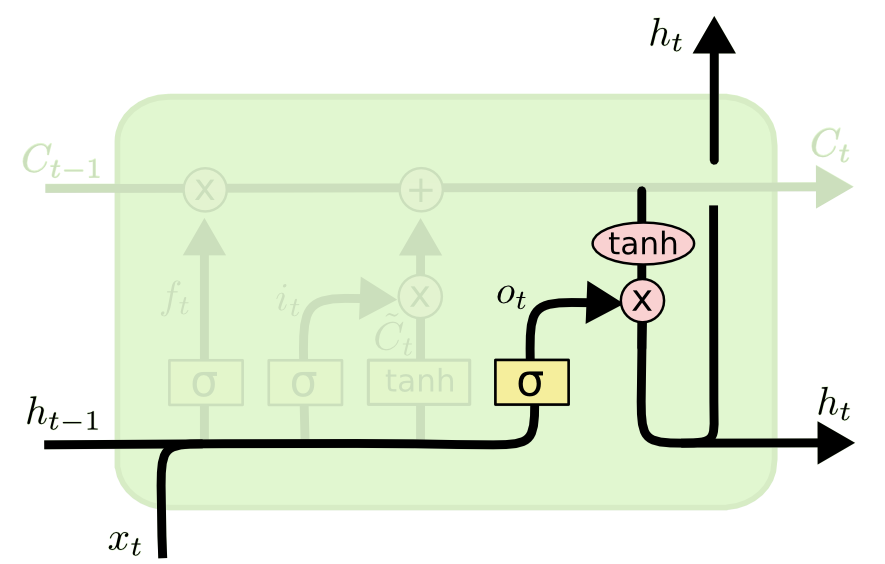
• The output gate decides which part of the new state will be used for the output.

\mathbf{o}_t = \sigma(W_o \times [\mathbf{h}_{t-1}; \mathbf{x}_t] + \mathbf{b}_o)

• The output not only influences the decision, but also how the gates will updated at the next step.

\mathbf{h}_t = \mathbf{o}_t \odot \text{tanh} (\mathbf{C}_t)

LSTM

• The function between \mathbf{x}_t and \mathbf{h}_t is quite complicated, with many different weights, but everything is differentiable: BPTT can be applied.

Source: http://colah.github.io/posts/2015-08-Understanding-LSTMs

Forget gate

\mathbf{f}_t = \sigma(W_f \times [\mathbf{h}_{t-1}; \mathbf{x}_t] + \mathbf{b}_f)

Input gate

\mathbf{i}_t = \sigma(W_i \times [\mathbf{h}_{t-1}; \mathbf{x}_t] + \mathbf{b}_i)

Output gate

\mathbf{o}_t = \sigma(W_o \times [\mathbf{h}_{t-1}; \mathbf{x}_t] + \mathbf{b}_o)

Candidate state

\tilde{\mathbf{C}}_t = \text{tanh}(W_C \times [\mathbf{h}_{t-1}; \mathbf{x}_t] + \mathbf{b}_c)

New state

\mathbf{C}_t = \mathbf{f}_t \odot \mathbf{C}_{t-1} + \mathbf{i}_t \odot \tilde{\mathbf{C}}_t

Output

\mathbf{h}_t = \mathbf{o}_t \odot \text{tanh} (\mathbf{C}_t)

How do LSTM solve the vanishing gradient problem?

Source: http://colah.github.io/posts/2015-08-Understanding-LSTMs

• Not all inputs are remembered by the LSTM: the input gate controls what comes in.

• If only \mathbf{x}_0 and \mathbf{x}_1 are needed to produce \mathbf{h}_{t+1}, they will be the only ones stored in the state, the other inputs are ignored.

How do LSTM solve the vanishing gradient problem?

Source: http://colah.github.io/posts/2015-08-Understanding-LSTMs

• If the state stays constant between t=1 and t, the gradient of the error will not vanish when backpropagating from t to t=1, because nothing happens!

\mathbf{C}_t = \mathbf{C}_{t-1} \rightarrow \frac{\partial \mathbf{C}_t}{\partial \mathbf{C}_{t-1}} = 1

• The gradient is multiplied by exactly one when the gates are closed.

LSTM networks

• LSTM are particularly good at learning long-term dependencies, because the gates protect the cell from vanishing gradients.

• Its problem is how to find out which inputs (e.g. \mathbf{x}_0 and \mathbf{x}_1) should enter or leave the state memory.

• Truncated BPTT is used to train all weights: the weights for the candidate state (as for RNN), and the weights of the three gates.

• LSTM are also subject to overfitting. Regularization (including dropout) can be used.

• The weights (also for the gates) can be convolutional.

• The gates also have a bias, which can be fixed (but hard to find).

• LSTM layers can be stacked to detect dependencies at different scales (deep LSTM network).

Peephole connections

Source: http://colah.github.io/posts/2015-08-Understanding-LSTMs

• A popular variant of LSTM adds peephole connections, where the three gates have additionally access to the state \mathbf{C}_{t-1}.

\mathbf{f}_t = \sigma(W_f \times [\mathbf{C}_{t-1}; \mathbf{h}_{t-1}; \mathbf{x}_t] + \mathbf{b}_f)

\mathbf{i}_t = \sigma(W_i \times [\mathbf{C}_{t-1}; \mathbf{h}_{t-1}; \mathbf{x}_t] + \mathbf{b}_i)

\mathbf{o}_t = \sigma(W_o \times [\mathbf{C}_{t}; \mathbf{h}_{t-1}; \mathbf{x}_t] + \mathbf{b}_o)

• It usually works better, but it adds more weights.

GRU: Gated Recurrent Unit

• Another variant is called the Gated Recurrent Unit (GRU).

• It uses directly the output \mathbf{h}_t as a state, and the forget and input gates are merged into a single gate \mathbf{r}_t.

\mathbf{z}_t = \sigma(W_z \times [\mathbf{h}_{t-1}; \mathbf{x}_t])

\mathbf{r}_t = \sigma(W_r \times [\mathbf{h}_{t-1}; \mathbf{x}_t])

\tilde{\mathbf{h}}_t = \text{tanh} (W_h \times [\mathbf{r}_t \odot \mathbf{h}_{t-1}; \mathbf{x}_t])

\mathbf{h}_t = (1 - \mathbf{z}_t) \odot \mathbf{h}_{t-1} + \mathbf{z}_t \odot \tilde{\mathbf{h}}_t

Source: http://colah.github.io/posts/2015-08-Understanding-LSTMs

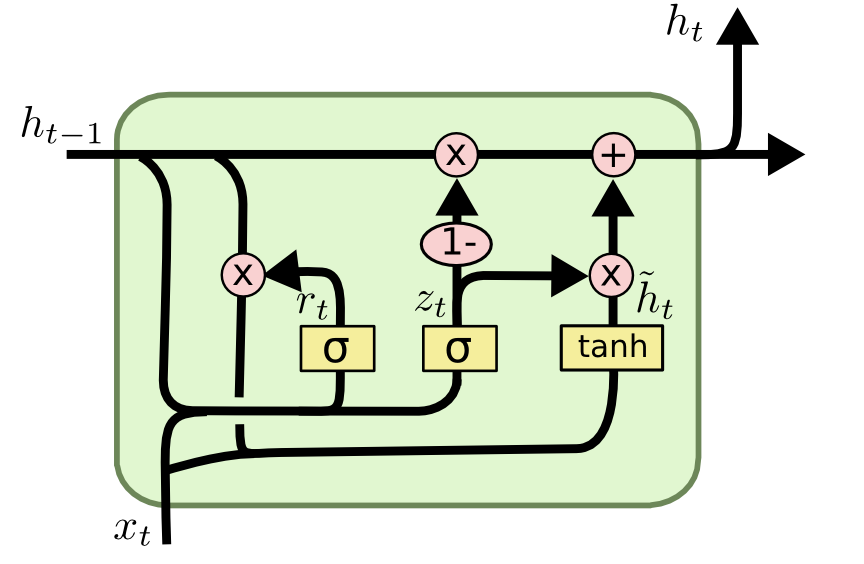
• It does not even need biases (mostly useless in LSTMs anyway).

• Much simpler to train as the LSTM, and almost as powerful.

Bidirectional LSTM

Source: http://www.paddlepaddle.org/doc/demo/sentiment_analysis/sentiment_analysis.html

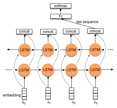
• A bidirectional LSTM learns to predict the output in two directions:

  • The feedforward line learns using the past context (classical LSTM).

  • The backforward line learns using the future context (inputs are reversed).

• The two state vectors are then concatenated at each time step to produce the output.

• Only possible offline, as the future inputs must be known.

• Works better than LSTM on many problems, but slower.

References

• A great blog post by Christopher Olah to understand recurrent neural networks, especially LSTM:

http://colah.github.io/posts/2015-08-Understanding-LSTMs

• Shi Yan built on that post to explain it another way:

https://medium.com/@shiyan/understanding-lstm-and-its-diagrams-37e2f46f1714#.m7fxgvjwf