5 Advantage Actor-Critic methods
The policy gradient theorem provides an actor-critic architecture able to learn parameterized policies. In comparison to REINFORCE, the policy gradient depends on the Q-values of the actions taken during the trajectory rather than on the obtained returns \(R(\tau)\). Quite obviously, it will also suffer from the high variance of the gradient, requiring the use of baselines. In this section, the baseline is state-dependent and chosen equal to the value of the state \(V^\pi(s)\), so the factor multiplying the log-likelihood of the policy is:
\[ A^{\pi}(s, a) = Q^{\pi}(s, a) - V^\pi(s) \]
which is the advantage of the action \(a\) in \(s\), as already seen in duelling networks.
Now the problem is that the critic would have to approximate two functions: \(Q^{\pi}(s, a)\) and \(V^{\pi}(s)\). Advantage actor-critic methods presented in this section (A2C, A3C, GAE) approximate the advantage of an action:
\[ \nabla_\theta J(\theta) = \mathbb{E}_{s \sim \rho^\pi, a \sim \pi_\theta}[\nabla_\theta \log \pi_\theta(s, a) \, A_\varphi(s, a)] \]
\(A_\varphi(s, a)\) is called the advantage estimate and should be equal to the real advantage in expectation.
Different methods could be used to compute the advantage estimate:
\(A_\varphi(s, a) = R(s, a) - V_\varphi(s)\) is the MC advantage estimate, the Q-value of the action being replaced by the actual return.
\(A_\varphi(s, a) = r(s, a, s') + \gamma \, V_\varphi(s') - V_\varphi(s)\) is the TD advantage estimate or TD error.
\(A_\varphi(s, a) = \sum_{k=0}^{n-1} \gamma^{k} \, r_{t+k+1} + \gamma^n \, V_\varphi(s_{t+n+1}) - V_\varphi(s_t)\) is the n-step advantage estimate.
The most popular approach is the n-step advantage, which is at the core of the methods A2C and A3C, and can be understood as a trade-off between MC and TD. MC and TD advantages could be used as well, but come with the respective disadvantages of MC (need for finite episodes, slow updates) and TD (unstable). Generalized Advantage Estimation (GAE) takes another interesting approach to estimate the advantage.
Note: A2C is actually derived from the A3C algorithm presented later, but it is simpler to explain it first. See https://blog.openai.com/baselines-acktr-a2c/ for an explanation of the reasons. A good explanation of A2C and A3C with Python code is available at https://cgnicholls.github.io/reinforcement-learning/2017/03/27/a3c.html.
5.0.1 Advantage Actor-Critic (A2C)
The first aspect of A2C is that it relies on n-step updating, which is a trade-off between MC and TD:
- MC waits until the end of an episode to update the value of an action using the reward to-go (sum of obtained rewards) \(R(s, a)\).
- TD updates immediately the action using the immediate reward \(r(s, a, s')\) and approximates the rest with the value of the next state \(V^\pi(s)\).
- n-step uses the \(n\) next immediate rewards and approximates the rest with the value of the state visited \(n\) steps later.
\[ \nabla_\theta J(\theta) = \mathbb{E}_{s_t \sim \rho^\pi, a_t \sim \pi_\theta}[\nabla_\theta \log \pi_\theta(s_t, a_t) \, ( \sum_{k=0}^{n-1} \gamma^{k} \, r_{t+k+1} + \gamma^n \, V_\varphi(s_{t+n+1}) - V_\varphi(s_t))] \tag{5.1}\]
TD can be therefore be seen as a 1-step algorithm. For sparse rewards (mostly zero, +1 or -1 at the end of a game for example), this allows to update the \(n\) last actions which lead to a win/loss, instead of only the last one in TD, speeding up learning. However, there is no need for finite episodes as in MC. In other words, n-step estimation ensures a trade-off between bias (wrong updates based on estimated values as in TD) and variance (variability of the obtained returns as in MC). An alternative to n-step updating is the use of eligibility traces (see Sutton and Barto (1998)).
A2C has an actor-critic architecture (Figure 5.1):
- The actor outputs the policy \(\pi_\theta\) for a state \(s\), i.e. a vector of probabilities for each action.
- The critic outputs the value \(V_\varphi(s)\) of a state \(s\).

Having a computable formula for the policy gradient, the algorithm is rather simple:
Acquire a batch of transitions \((s, a, r, s')\) using the current policy \(\pi_\theta\) (either a finite episode or a truncated one).
For each state encountered, compute the discounted sum of the next \(n\) rewards \(\sum_{k=0}^{n} \gamma^{k} \, r_{t+k+1}\) and use the critic to estimate the value of the state encountered \(n\) steps later \(V_\varphi(s_{t+n+1})\).
\[ R_t = \sum_{k=0}^{n-1} \gamma^{k} \, r_{t+k+1} + \gamma^n \, V_\varphi(s_{t+n+1}) \]
- Update the actor using Equation 5.1.
\[ \nabla_\theta J(\theta) = \sum_t \nabla_\theta \log \pi_\theta(s_t, a_t) \, (R_t - V_\varphi(s_t)) \]
- Update the critic to minimize the TD error between the estimated value of a state and its true value.
\[ \mathcal{L}(\varphi) = \sum_t (R_t - V_\varphi(s_t))^2 \]
- Repeat.
This is not very different in essence from REINFORCE (sample transitions, compute the return, update the policy), apart from the facts that episodes do not need to be finite and that a critic has to be learned in parallel. A more detailed pseudo-algorithm for a single A2C learner is the following:
- Initialize the actor \(\pi_\theta\) and the critic \(V_\varphi\) with random weights.
- Observe the initial state \(s_0\).
- for \(t \in [0, T_\text{total}]\):
Initialize empty episode minibatch.
for \(k \in [0, n]\): # Sample episode
- Select a action \(a_k\) using the actor \(\pi_\theta\).
- Perform the action \(a_k\) and observe the next state \(s_{k+1}\) and the reward \(r_{k+1}\).
- Store \((s_k, a_k, r_{k+1})\) in the episode minibatch.
if \(s_n\) is not terminal: set \(R = V_\varphi(s_n)\) with the critic, else \(R=0\).
Reset gradient \(d\theta\) and \(d\varphi\) to 0.
for \(k \in [n-1, 0]\): # Backwards iteration over the episode
- Update the discounted sum of rewards \(R = r_k + \gamma \, R\)
- Accumulate the policy gradient using the critic: \[ d\theta \leftarrow d\theta + \nabla_\theta \log \pi_\theta(s_k, a_k) \, (R - V_\varphi(s_k)) \]
- Accumulate the critic gradient: \[ d\varphi \leftarrow d\varphi + \nabla_\varphi (R - V_\varphi(s_k))^2 \]
Update the actor and the critic with the accumulated gradients using gradient descent or similar: \[ \theta \leftarrow \theta + \eta \, d\theta \qquad \varphi \leftarrow \varphi + \eta \, d\varphi \]
Note that not all states are updated with the same horizon \(n\): the last action encountered in the sampled episode will only use the last reward and the value of the final state (TD learning), while the very first action will use the \(n\) accumulated rewards. In practice it does not really matter, but the choice of the discount rate \(\gamma\) will have a significant influence on the results.
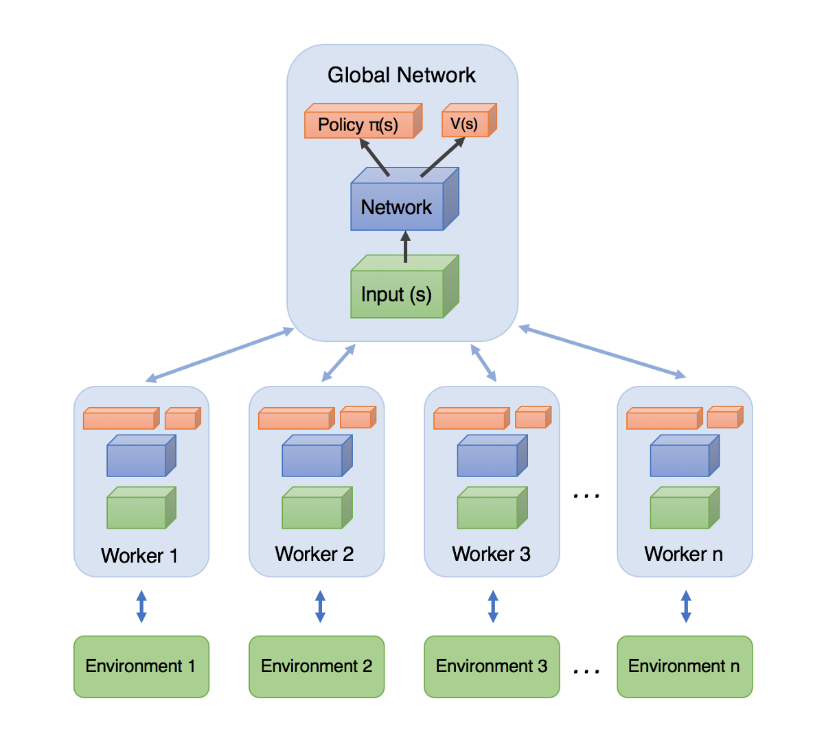
As many actor-critic methods, A2C performs online learning: a couple of transitions are explored using the current policy, which is immediately updated. As for value-based networks (e.g. DQN), the underlying NN will be affected by the correlated inputs and outputs: a single batch contains similar states and action (e.g. consecutive frames of a video game). The solution retained in A2C and A3C does not depend on an experience replay memory as DQN, but rather on the use of multiple parallel actors and learners.
The idea is depicted on Figure 5.2 (actually for A3C, but works with A2C). The actor and critic are stored in a global network. Multiple instances of the environment are created in different parallel threads (the workers or actor-learners). At the beginning of an episode, each worker receives a copy of the actor and critic weights from the global network. Each worker samples an episode (starting from different initial states, so the episodes are uncorrelated), computes the accumulated gradients and sends them back to the global network. The global networks merges the gradients and uses them to update the parameters of the policy and critic networks. The new parameters are send to each worker again, until it converges.
- Initialize the actor \(\pi_\theta\) and the critic \(V_\varphi\) in the global network.
- repeat:
- for each worker \(i\) in parallel:
- Get a copy of the global actor \(\pi_\theta\) and critic \(V_\varphi\).
- Sample an episode of \(n\) steps.
- Return the accumulated gradients \(d\theta_i\) and \(d\varphi_i\).
- Wait for all workers to terminate.
- Merge all accumulated gradients into \(d\theta\) and \(d\varphi\).
- Update the global actor and critic networks.
- for each worker \(i\) in parallel:
This solves the problem of correlated inputs and outputs, as each worker explores different regions of the environment (one can set different initial states in each worker, vary the exploration rate, etc), so the final batch of transitions used for training the global networks is much less correlated. The only drawback of this approach is that it has to be possible to explore multiple environments in parallel. This is easy to achieve in simulated environments (e.g. video games) but much harder in real-world systems like robots. A brute-force solution for robotics is simply to buy enough robots and let them learn in parallel (Gu et al., 2017).
5.0.2 Asynchronous Advantage Actor-Critic (A3C)
Asynchronous Advantage Actor-Critic (A3C, Mnih et al., 2016) extends the approach of A2C by removing the need of synchronization between the workers at the end of each episode before applying the gradients. The rationale behind this is that each worker may need different times to complete its task, so they need to be synchronized. Some workers might then be idle most of the time, what is a waste of resources. Gradient merging and parameter updates are sequential operations, so no significant speedup is to be expected even if one increases the number of workers.
The solution retained in A3C is to simply skip the synchronization step: each worker reads and writes the network parameters whenever it wants. Without synchronization barriers, there is of course a risk that one worker tries to read the network parameters while another writes them: the obtained parameters would be a mix of two different networks. Surprisingly, it does not matter: if the learning rate is small enough, there is anyway not a big difference between two successive versions of the network parameters. This kind of “dirty” parameter sharing is called HogWild! updating (Niu et al., 2011) and has been proven to work under certain conditions which are met here.
The resulting A3C pseudocode is summarized here:
Initialize the actor \(\pi_\theta\) and the critic \(V_\varphi\) in the global network.
for each worker \(i\) in parallel:
- repeat:
- Get a copy of the global actor \(\pi_\theta\) and critic \(V_\varphi\).
- Sample an episode of \(n\) steps.
- Compute the accumulated gradients \(d\theta_i\) and \(d\varphi_i\).
- Update the global actor and critic networks asynchronously (HogWild!).
- repeat:
The workers are fully independent: their only communication is through the asynchronous updating of the global networks. This can lead to very efficient parallel implementations: in the original A3C paper (Mnih et al., 2016), they solved the same Atari games than DQN using 16 CPU cores instead of a powerful GPU, while achieving a better performance in less training time (1 day instead of 8). The speedup is almost linear: the more workers, the faster the computations, the better the performance (as the policy updates are less correlated).
Entropy regularization
An interesting addition in A3C is the way they enforce exploration during learning. In actor-critic methods, exploration classically relies on the fact that the learned policies are stochastic (on-policy): \(\pi(s, a)\) describes the probability of taking the action \(a\) in the state \(s\). In discrete action spaces, the output of the actor is usually a softmax layer, ensuring that all actions get a non-zero probability of being selected during training. In continuous action spaces, the executed action is sampled from the output probability distribution. However, this is often not sufficient and hard to control.
In A3C, the authors added an entropy regularization term (Williams and Peng, 1991) to the policy gradient update:
\[ \nabla_\theta J(\theta) = \mathbb{E}_{s_t \sim \rho^\pi, a_t \sim \pi_\theta}[\nabla_\theta \log \pi_\theta(s_t, a_t) \, ( R_t - V_\varphi(s_t)) + \beta \, \nabla_\theta H(\pi_\theta(s_t))] \tag{5.2}\]
For discrete actions, the entropy of the policy for a state \(s_t\) is simple to compute: \(H(\pi_\theta(s_t)) = - \sum_a \pi_\theta(s_t, a) \, \log \pi_\theta(s_t, a)\). For continuous actions, replace the sum with an integral. It measures the “randomness” of the policy: if the policy is fully deterministic (the same action is systematically selected), the entropy is zero as it carries no information. If the policy is completely random, the entropy is maximal. Maximizing the entropy at the same time as the returns improves exploration by forcing the policy to be as non-deterministic as possible.
The parameter \(\beta\) controls the level of regularization: we do not want the entropy to dominate either, as a purely random policy does not bring much reward. If \(\beta\) is chosen too low, the entropy won’t play a significant role in the optimization and we may obtain a suboptimal deterministic policy early during training as there was not enough exploration. If \(\beta\) is too high, the policy will be random. Entropy regularization adds yet another hyperparameter to the problem, but can be really useful for convergence when adequately chosen.
Comparison between A3C and DQN
- DQN uses an experience replay memory to solve the correlation of inputs/outputs problem, while A3C uses parallel actor-learners. If multiple copies of the environment are available, A3C should be preferred because the ERM slows down learning (very old transitions are still used for learning) and requires a lot of memory.
- A3C is on-policy: the learned policy must be used to explore the environment. DQN is off-policy: a behavior policy can be used for exploration, allowing to guide externally which regions of the state-action space should be explored. Off-policy are often preferred when expert knowledge is available.
- DQN has to use target networks to fight the non-stationarity of the Q-values. A3C uses state-values and advantages, which are much more stable over time than Q-values, so there is no need for target networks.
- A3C can deal with continuous action spaces easily, as it uses a parameterized policy. DQN has to be strongly modified to deal with this problem.
- Both can deal with POMDP by using LSTMs in the actor network: A3C (Mirowski et al., 2016; Mnih et al., 2016), DQN (Hausknecht and Stone, 2015).
5.0.3 Generalized Advantage Estimation (GAE)
The different versions of the policy gradient seen so far take the form:
\[ \nabla_\theta J(\theta) = \mathbb{E}_{s_t \sim \rho^\pi, a_t \sim \pi_\theta}[\nabla_\theta \log \pi_\theta (s_t, a_t) \, \psi_t ] \]
where:
\(\psi_t = R_t\) is the REINFORCE algorithm (MC sampling).
\(\psi_t = R_t - b\) is the REINFORCE with baseline algorithm.
\(\psi_t = Q^\pi(s_t, a_t)\) is the policy gradient theorem.
\(\psi_t = A^\pi(s_t, a_t)\) is the advantage actor critic.
\(\psi_t = r_{t+1} + \gamma \, V^\pi(s_{t+1}) - V^\pi(s_t)\) is the TD actor critic.
\(\psi_t = \sum_{k=0}^{n-1} \gamma^{k} \, r_{t+k+1} + \gamma^n \, V^\pi(s_{t+n+1}) - V^\pi(s_t)\) is the n-step algorithm (A2C).
Generally speaking:
- the more \(\psi_t\) relies on real rewards (e.g. \(R_t\)), the more the gradient will be correct on average (small bias), but the more it will vary (high variance). This increases the sample complexity: we need to average more samples to correctly estimate the gradient.
- the more \(\psi_t\) relies on estimations (e.g. the TD error), the more stable the gradient (small variance), but the more incorrect it is (high bias). This can lead to suboptimal policies, i.e. local optima of the objective function.
This is the classical bias/variance trade-off in machine learning. The n-step algorithm used in A2C is an attempt to mitigate between these extrema. Schulman et al. (2015) proposed the Generalized Advantage Estimate (GAE) to further control the bias/variance trade-off.
Let’s define the n-step advantage:
\[ A^{n}_t = \sum_{k=0}^{n-1} \gamma^{k} \, r_{t+k+1} + \gamma^n \, V^\pi(s_{t+n+1}) - V^\pi(s_t) \]
It is easy to show recursively that it depends on the TD error \(\delta_t = r_{t+1} + \gamma \, V^\pi(s_{t+1}) - V^\pi(s_t)\) of the \(n\) next steps:
\[ A^{n}_t = \sum_{l=0}^{n-1} \gamma^l \, \delta_{t+l} \]
In other words, the prediction error over \(n\) steps is the (discounted) sum of the prediction errors between two successive steps. Now, what is the optimal value of \(n\)? GAE decides not to choose and to simply average all n-step advantages and to weight them with a discount parameter \(\lambda\). This defines the Generalized Advantage Estimator \(A^{\text{GAE}(\gamma, \lambda)}_t\):
\[ A^{\text{GAE}(\gamma, \lambda)}_t = (1-\lambda) \, \sum_{l=0}^\infty \lambda^l A^l_t = \sum_{l=0}^\infty (\gamma \lambda)^l \delta_{t+l} \]
The GAE is the discounted sum of all n-step advantages. When \(\lambda=0\), we have \(A^{\text{GAE}(\gamma, 0)}_t = A^{0}_t = \delta_t\), i.e. the TD advantage (high bias, low variance). When \(\lambda=1\), we have (at the limit) \(A^{\text{GAE}(\gamma, 1)}_t = R_t\), i.e. the MC advantage (low bias, high variance). Choosing the right value of \(\lambda\) between 0 and 1 allows to control the bias/variance trade-off.
\(\gamma\) and \(\lambda\) play different roles in GAE: \(\gamma\) determines the scale or horizon of the value functions: how much future rewards rewards are to be taken into account. The higher \(\gamma <1\), the smaller the bias, but the higher the variance. Empirically, Schulman et al. (2015) found that small \(\lambda\) values introduce less bias than \(\gamma\), so \(\lambda\) can be chosen smaller than \(\gamma\) (which is typically 0.99).
The policy gradient for Generalized Advantage Estimation is therefore:
\[ \nabla_\theta J(\theta) = \mathbb{E}_{s_t \sim \rho^\pi, a_t \sim \pi_\theta}[\nabla_\theta \log \pi_\theta (s_t, a_t) \, \sum_{l=0}^\infty (\gamma \lambda)^l \delta_{t+l} ] \]
Note that Schulman et al. (2015) additionally use trust region optimization to stabilize learning and further reduce the bias, for now just consider it is a better optimization method than gradient descent. The GAE algorithm is summarized here:
- Initialize the actor \(\pi_\theta\) and the critic \(V_\varphi\) with random weights.
- for \(t \in [0, T_\text{total}]\):
Initialize empty minibatch.
for \(k \in [0, n]\):
- Select a action \(a_k\) using the actor \(\pi_\theta\).
- Perform the action \(a_k\) and observe the next state \(s_{k+1}\) and the reward \(r_{k+1}\).
- Store \((s_k, a_k, r_{k+1})\) in the minibatch.
for \(k \in [0, n]\):
- Compute the TD error \(\delta_k = r_{k+1} + \gamma \, V_\varphi(s_{k+1}) - V_\varphi(s_k)\)
for \(k \in [0, n]\):
- Compute the GAE advantage \(A^{\text{GAE}(\gamma, \lambda)}_k = \sum_{l=0}^\infty (\gamma \lambda)^l \delta_{k+l}\)
Update the actor using the GAE advantage and natural gradients (TRPO).
Update the critic using natural gradients (TRPO)
5.0.4 Stochastic actor-critic for continuous action spaces
The actor-critic method presented above use stochastic policies \(\pi_\theta(s, a)\) assigning parameterized probabilities of being selecting to each \((s, a)\) pair.
When the action space is discrete, the output layer of the actor is simply a softmax layer with as many neurons as possible actions in each state, making sure the probabilities sum to one. It is then straightforward to sample an action from this layer.
When the action space is continuous (e.g. the different joints of a robotic arm), one has to make an assumption on the underlying distribution. The actor learns the parameters of the distribution (for example the mean and variance of a Gaussian distribution) and the executed action is simply sampled from the parameterized distribution.
The most used distribution is the Gaussian distribution, leading to Gaussian policies. In this case, the output of the actor is a mean vector \(\mu_\theta(s)\) and possibly a variance vector \(\sigma_\theta(s)\). The policy is then simply defined as:
\[ \pi_\theta(s, a) = \frac{1}{\sqrt{2\pi\sigma^2_\theta(s)}} \, \exp -\frac{(a - \mu_\theta(s))^2}{2\sigma_\theta(s)^2} \]
In order to use backpropagation on the policy gradient (i.e. getting an analytical form of the score function \(\nabla_\theta \log \pi_\theta (s, a)\)), one can use the re-parameterization trick (Heess et al., 2015) by rewriting the policy as:
\[ a = \mu_\theta(s) + \sigma_\theta(s) \times \xi \qquad \text{where} \qquad \xi \sim \mathcal{N}(0,1) \]
To select an action, we only need to sample \(\xi\) from the unit normal distribution, multiply it by the standard deviation and add the mean. To compute the score function, we use the following partial derivatives:
\[ \nabla_\mu \log \pi_\theta (s, a) = \frac{a - \mu_\theta(s)}{\sigma_\theta(s)^2} \qquad \nabla_\sigma \log \pi_\theta (s, a) = \frac{(a - \mu_\theta(s))^2}{\sigma_\theta(s)^3} - \frac{1}{\sigma_\theta(s)} \]
and use the chain rule to obtain the score function. The re-parameterization trick is a cool trick to apply backpropagation on stochastic problems: it is for example used in the variational auto-encoders [VAE;Kingma and Welling (2013)].
Depending on the problem, one could use: 1) a fixed \(\sigma\) for the whole action space, 2) a fixed \(\sigma\) per DoF, 3) a learnable \(\sigma\) per DoF (assuming all action dimensions to be mutually independent) or even 4) a covariance matrix \(\Sigma\) when the action dimensions are dependent.
One limitation of Gaussian policies is that their support is infinite: even with a small variance, samples actions can deviate a lot (albeit rarely) from the mean. This is particularly a problem when action must have a limited range: the torque of an effector, the linear or angular speed of a car, etc. Clipping the sampled action to minimal and maximal values introduces a bias which can impair learning. Chou et al. (2017) proposed to use beta-distributions instead of Gaussian ones in the actor. Sampled values have a \([0,1]\) support, which can rescaled to \([v_\text{min},v_\text{max}]\) easily. They show that beta policies have less bias than Gaussian policies in most continuous problems.