FORCE learning of the readout weights

import numpy as np
import matplotlib.pyplot as plt

import water_tank as wt

Let’s first generate the Mackey-Glass data:

from reservoirpy.datasets import mackey_glass

# Generate time series
mg = mackey_glass(4000, x0=1.2)

# Normalize between -1 and 1
mg =  2.0 * (mg - mg.min()) / (mg.max() - mg.min()) - 1.0

# The task is to predict the next value
X = mg[:-1, 0]
Y = mg[1:, 0]

plt.figure(figsize=(12, 7))
plt.plot(X)
plt.xlabel("Time (ms)")
plt.title("Mackey-Glass time series")
plt.show()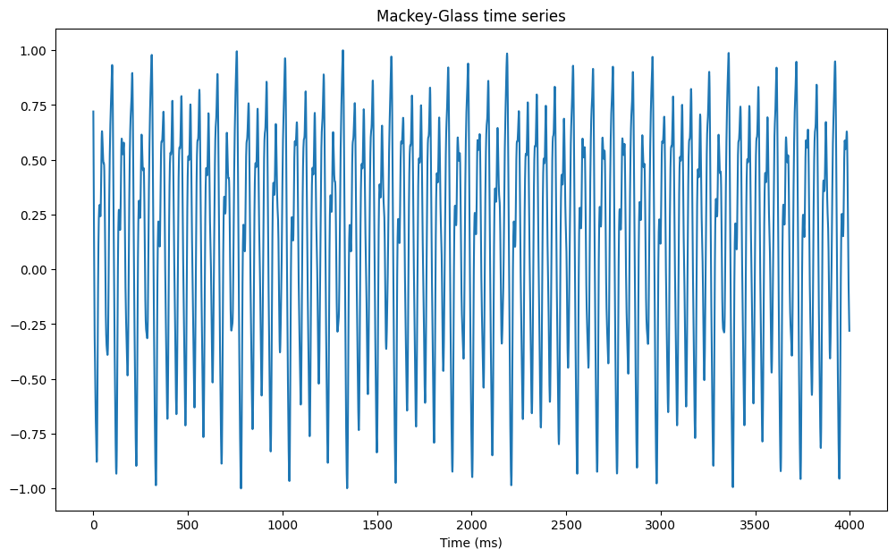

To implement FORCE learning, we create an echo-state network with:

• a reservoir with N tanh neurons.
• a readout layer with one neuron, with feedback to the reservoir.

The weight matrices are initialized classically.

The readout weights are trained online using the recursive least squares (RLS) method as before.

class ESN(object):

    def __init__(self, N, N_out, g, tau, sparseness):

        # Reservoir 
        self.rc = wt.layers.RecurrentLayer(size=N, tau=tau)

        # Readout
        self.readout = wt.layers.LinearReadout(size=N_out)

        # Recurrent projection
        self.rec_proj = wt.connect(
            pre = self.rc, 
            post = self.rc, 
            weights = wt.random.Normal(0.0, g/np.sqrt(sparseness*N)), 
            bias = wt.random.Bernouilli([-1.0, 1.0], p=0.5),
            sparseness = sparseness)

        # Readout projection
        self.readout_proj = wt.connect(
            pre = self.rc, 
            post = self.readout,
            weights = wt.random.Const(0.0),
            bias = wt.random.Const(0.0), # learnable bias
            sparseness = 1.0 # readout should be dense
        )

        # Feedback projection
        self.feedback_proj = wt.connect(self.readout, self.rc, wt.random.Uniform(-1.0, 1.0))

        # Learning rules
        self.learningrule = wt.rules.RLS(projection=self.readout_proj, delta=1e-6)

        # Recorder
        self.recorder = wt.Recorder()

    @wt.measure
    def train(self, X, warmup=0):

        for t, x in enumerate(X): 

            # Steps 
            self.rc.step() 
            self.readout.step()

            # Learning
            if t >= warmup: self.learningrule.train(error= np.array([x]) - self.readout.output())

            # Recording
            self.recorder.record({
                'rc': self.rc.output(), 
                'readout': self.readout.output(),
            })
    
    @wt.measure
    def autoregressive(self, duration):

        for _ in range(duration): 

            # Steps 
            self.rc.step() 
            self.readout.step()

            # Recording
            self.recorder.record({
                'rc': self.rc.output(), 
                'readout': self.readout.output()
            })

N_out = 1 # number of outputs
N = 200 # number of neurons
g = 1.25 # scaling factor
tau = 3.3 # time constant
sparseness = 0.1 # sparseness of the recurrent weights

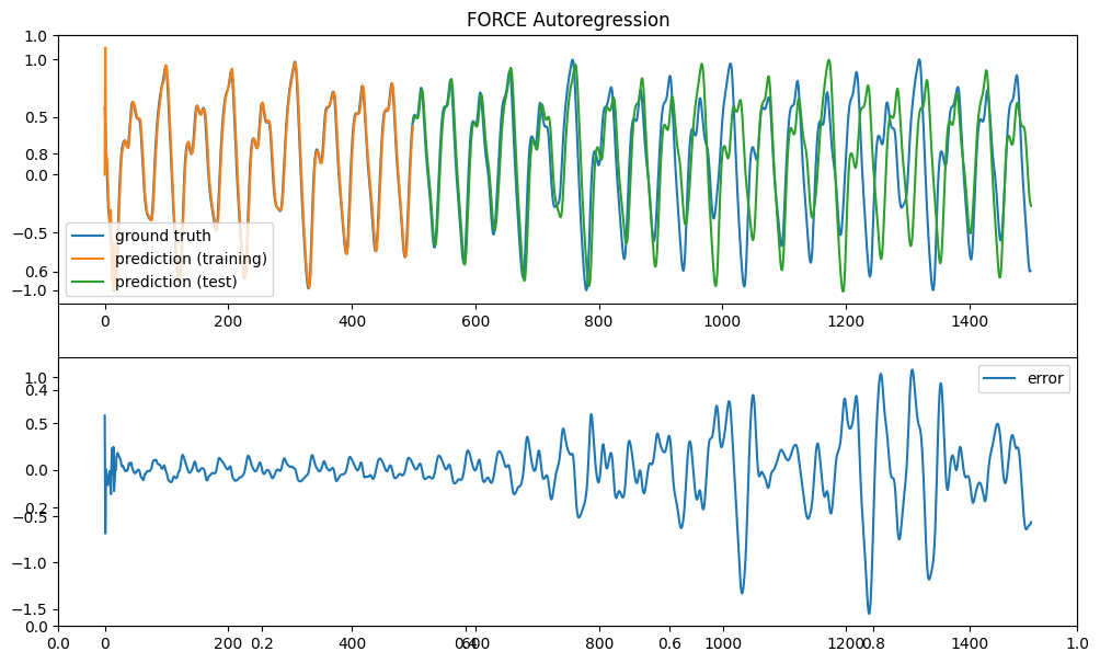
net = ESN(N, N_out, g, tau, sparseness)

We train the reservoir for 500 time steps and let it predict the signal autoregressively for 1000 steps.

# Training / test
d_train = 500
d_test = 1000

# Supervised training
net.train(X[:d_train], warmup=0)

# Autoregressive test
net.autoregressive(duration=d_test)

data = net.recorder.get()

Execution time: 43 ms
Execution time: 27 ms

The performance is quite comparable to the supervised RLS rule.

plt.figure(figsize=(12, 7))
plt.title("FORCE Autoregression")
plt.subplot(211)
plt.plot(Y[:d_train+d_test], label='ground truth')
plt.plot(data['readout'][:d_train], label='prediction (training)')
plt.plot(np.linspace(d_train, d_train+d_test, d_test), data['readout'][d_train:], label='prediction (test)')
plt.legend()
plt.subplot(212)
plt.plot(Y[:d_train+d_test] - data['readout'][:], label='error')
plt.legend()

plt.show()