import numpy as np
import matplotlib.pyplot as plt

import water_tank as wtMackey-Glass autoregression
The Mackey-Glass equations are delay differential equations that exhibit chaotic behavior, i.e. they cannot be predict accurately for a long period of time.
\frac{d x(t)}{dt} = \beta \, \frac{x(t - \tau)}{1 + x(t - \tau)^n} - \gamma \, x(t)
To check this, we use reservoirpy (https://reservoirpy.readthedocs.io) to generate two time series with very close initial conditions (\epsilon = 10^{-6}). After roughly two seconds of simulation, the two time series start to diverge.
from reservoirpy.datasets import mackey_glass

mg1 = mackey_glass(4000, x0=1.2)
mg2 = mackey_glass(4000, x0=1.2 + 1e-6)

plt.figure(figsize=(12, 7))
plt.plot(mg1, label="first")
plt.plot(mg2, label="second")
plt.plot(mg1 - mg2, label="difference")
plt.legend()
plt.xlabel("Time (ms)")
plt.title("Mackey-Glass time series")
plt.show()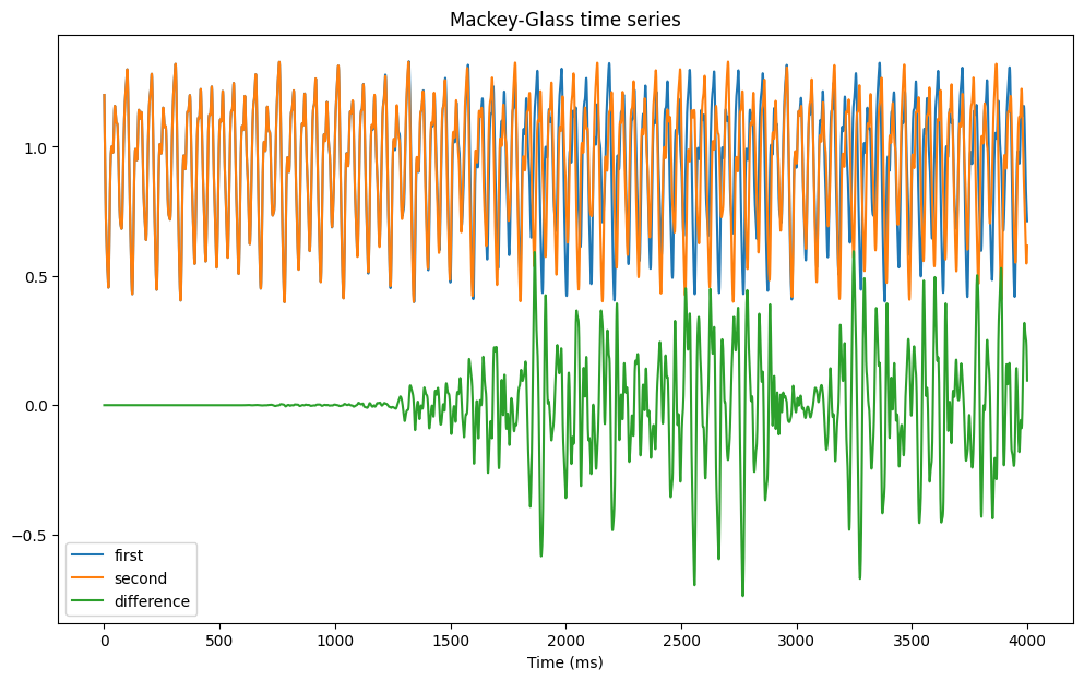
For the autoregression task, we generate a time series, normalize it and create supervised targets to predict the value of the signal at time t + 1 given the past.
# Generate time series
mg = mackey_glass(4000, x0=1.2)

# Normalize between -1 and 1
mg =  2.0 * (mg - mg.min()) / (mg.max() - mg.min()) - 1.0

# The task is to predict the next value
X = mg[:-1, 0]
Y = mg[1:, 0]

plt.figure(figsize=(12, 7))
plt.plot(X)
plt.xlabel("Time (ms)")
plt.title("Mackey-Glass time series")
plt.show()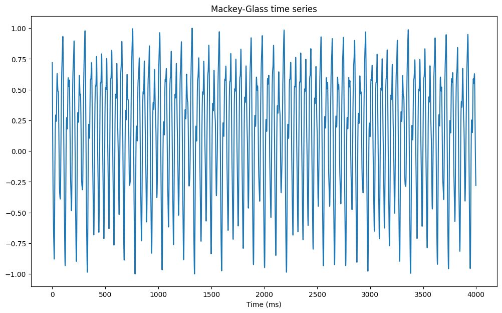
Using water-tank
We now create an echo-state network with:
- an input layer with one neuron
- a reservoir with N tanh neurons.
- a readout layer with one neuron.
The weight matrices are initialized classically. Note that the recurrent and readout neurons both use biases. The readout weights are trained online using the recursive least squares (RLS) method.
Two methods are implemented in the class: a training method calling the learning rule, and an autoregressive method plugging the output of the networks back into its input.
class ESN(object):

    def __init__(self, N, N_in, N_out, g, tau, sparseness):

        # Input population
        self.inp = wt.layers.StaticInput(size=N_in)

        # Reservoir
        self.rc = wt.layers.RecurrentLayer(size=N, tau=tau)

        # Readout
        self.readout = wt.layers.LinearReadout(size=N_out)

        # Input projection
        self.inp_proj = wt.connect(
            pre = self.inp,
            post = self.rc,
            weights = wt.random.Bernouilli([-1.0, 1.0], p=0.5),
            bias = None,
            sparseness = 0.1
        )

        # Recurrent projection
        self.rec_proj = wt.connect(
            pre = self.rc,
            post = self.rc,
            weights = wt.random.Normal(0.0, g/np.sqrt(sparseness*N)),
            bias = wt.random.Bernouilli([-1.0, 1.0], p=0.5), # very important
            sparseness = sparseness
        )

        # Readout projection
        self.readout_proj = wt.connect(
            pre = self.rc,
            post = self.readout,
            weights = wt.random.Const(0.0),
            bias = wt.random.Const(0.0), # learnable bias
            sparseness = 1.0 # readout should be dense
        )

        # Learning rules
        self.learningrule = wt.rules.RLS(
            projection=self.readout_proj,
            delta=1e-6
        )

        # Recorder
        self.recorder = wt.Recorder()

    @wt.measure
    def train(self, X, Y, warmup=0):

        for t, (x, y) in enumerate(zip(X, Y)):

            # Inputs/targets
            self.inp.set(x)

            # Steps
            self.rc.step()
            self.readout.step()

            # Learning
            if t >= warmup:
                self.learningrule.train(
                    error = y - self.readout.output()
                )

            # Recording
            self.recorder.record({
                'rc': self.rc.output(),
                'readout': self.readout.output(),
            })

    @wt.measure
    def autoregressive(self, duration):

        for _ in range(duration):
            # Autoregressive input
            self.inp.set(self.readout.output())

            # Steps
            self.rc.step()
            self.readout.step()

            # Recording
            self.recorder.record({
                'rc': self.rc.output(),
                'readout': self.readout.output()
            })
N_in = 1 # number of inputs
N_out = 1 # number of outputs
N = 200 # number of neurons
g = 1.25 # scaling factor
tau = 3.3 # time constant
sparseness = 0.1 # sparseness of the recurrent weights
net = ESN(N, N_in, N_out, g, tau, sparseness)We train the reservoir for 500 time steps and let it predict the signal autoregressively for 1000 steps.
# Training / test
d_train = 500
d_test = 1000

# Supervised training
net.train(X[:d_train], Y[:d_train], warmup=0)

# Autoregressive test
net.autoregressive(duration=d_test)

data = net.recorder.get()
Execution time: 70 ms
Execution time: 38 msThe training error becomes quickly very small. When predicting the time series autoregressively, the predictions are precise for around 200 steps, before starting to diverge.
plt.figure(figsize=(12, 7))
plt.subplot(211)
plt.title("Autoregression with water_tank")
plt.plot(Y[:d_train+d_test], label='ground truth')
plt.plot(data['readout'][:d_train], label='prediction (training)')
plt.plot(np.linspace(d_train, d_train+d_test, d_test), data['readout'][d_train:], label='prediction (test)')
plt.legend()
plt.subplot(212)
plt.plot(Y[:d_train+d_test] - data['readout'][:], label='error')
plt.legend()
plt.show()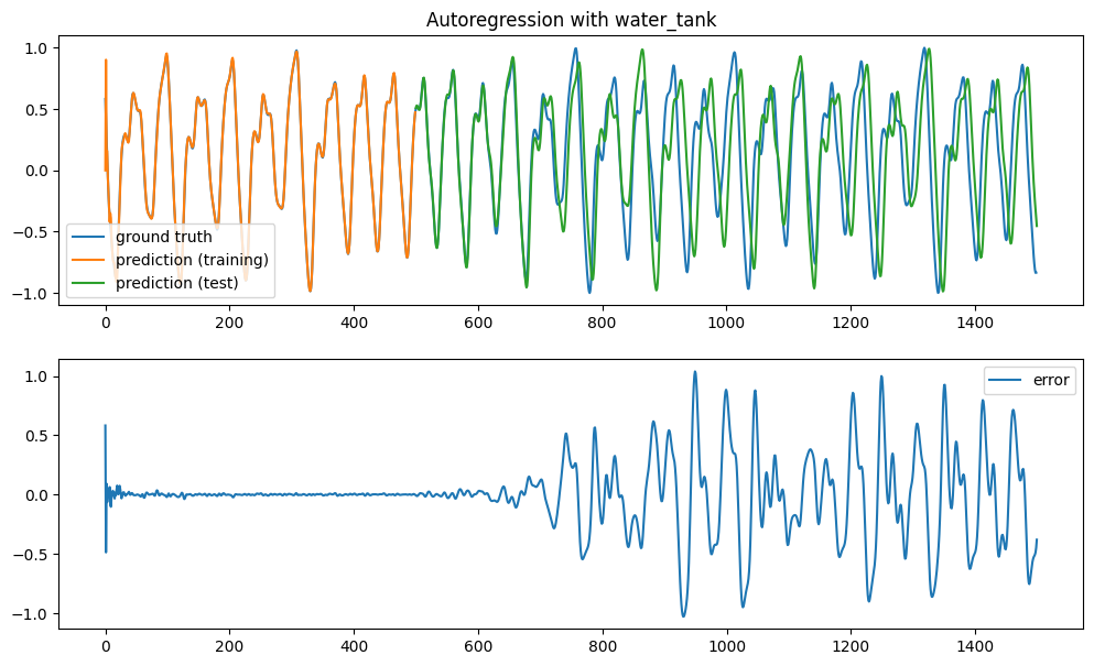
It is interesting to note that, for the autoregression to work correctly, the input biases are critical. They have the effect that many reservoir neurons are saturated (+1 or -1) and only a few are in the “useful” region and change their sign.
plt.figure(figsize=(12, 7))
plt.title("Reservoir activity")
for i in range(10):
    plt.plot(data['rc'][:, i])
plt.show()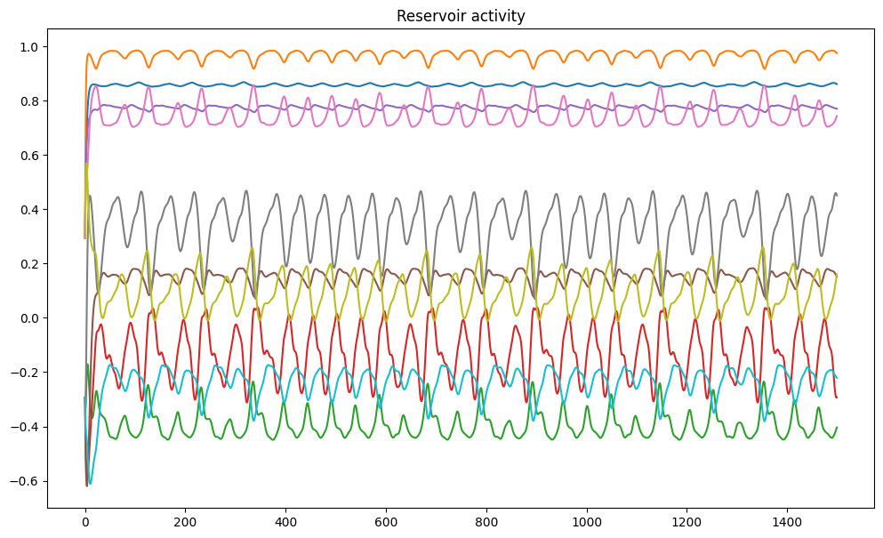
mean_act = data['rc'].mean(axis=0)

plt.figure(figsize=(12, 7))
plt.title("Mean neural activity during the training phase")
plt.hist(mean_act)
plt.show()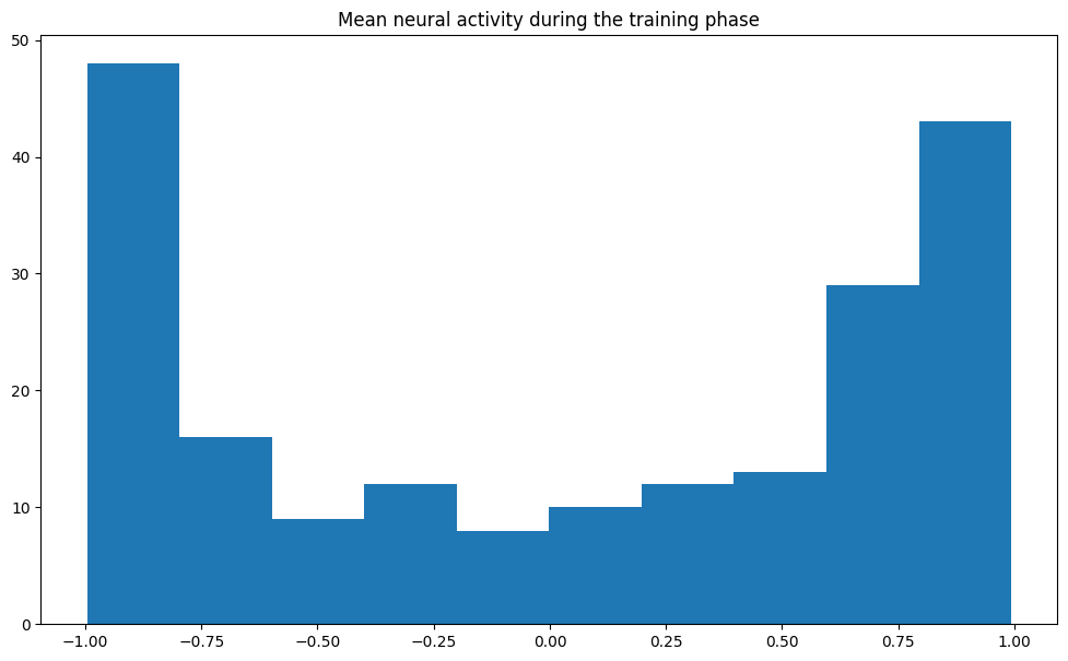
When plotting the readout weights after training, we can see that saturated neurons whose activity is very close to +1 or -1 throughout learning tend to get smaller readout weights. This is an effect of the inverse correlation matrix used in RLS: if the pre neuron is not significantly active, it should not participate to the output.
from sklearn.linear_model import LinearRegression
x = np.abs(mean_act).reshape((N, 1))
t = np.abs(net.readout_proj.W[0, :]).reshape((N, 1))
reg = LinearRegression().fit(x, t)
y = reg.predict([[0], [1]])

plt.figure(figsize=(12, 7))
plt.scatter(x, t)
plt.plot([0, 1], y)
plt.xlabel("Absolute activity")
plt.ylabel("Absolute weight")
plt.show()
--------------------------------------------------------------------------- ModuleNotFoundError Traceback (most recent call last) Cell In[10], line 1 ----> 1 from sklearn.linear_model import LinearRegression 2 x = np.abs(mean_act).reshape((N, 1)) 3 t = np.abs(net.readout_proj.W[0, :]).reshape((N, 1)) ModuleNotFoundError: No module named 'sklearn'
Using reservoirpy
For the sake of comparison, let’s see how the same problem is addressed by reservoirpy.
from reservoirpy.nodes import Reservoir, RLS
from reservoirpy.datasets import mackey_glass

# Mackey-Glass chaotic time series
X = mackey_glass(n_timesteps=2000)
X =  2.0 * (X - X.min()) / (X.max() - X.min()) - 1.0

# Create the reservoir with RLS online learning
reservoir = Reservoir(units=200, lr=0.3, sr=1.25)
readout = RLS(output_dim=1)
esn = reservoir >> readout

# Train / test
d_train = 500
d_test = 1000

# Supervised training
training = esn.train(X[:d_train], X[1:1+d_train])

# Autoregression
predictions = []
errors = list(X[1:1+d_train] - training)
pred = [X[d_train-1]]
for t in range(d_test):
    pred = esn.run(pred)
    predictions.append(pred[0])
    errors.append(X[d_train + t + 1, 0] - pred[0])

plt.figure(figsize=(12, 7))
plt.subplot(211)
plt.title("Autoregression with reservoirpy")
plt.plot(training, label='prediction (train)')
plt.plot(X[1:1+d_train], label='ground truth (train)')
plt.plot(np.arange(1+d_train, 1+d_train+d_test), predictions, label='prediction (test)')
plt.plot(np.arange(1+d_train, 1+d_train+d_test), X[1+d_train: 1+d_train+d_test, 0], label='ground truth (test)')
plt.legend()
plt.subplot(212)
plt.plot(errors, label='error')
plt.legend()
plt.show()