Temporal Difference learning
Temporal difference
The main drawback of Monte Carlo methods is that the task must be composed of finite episodes. Not only is it not always possible, but value updates have to wait for the end of the episode, what slows learning down.
Temporal difference methods simply replace the actual return obtained after a state or an action, by an estimation composed of the reward immediately received plus the value of the next state or action:
R_t \approx r(s, a, s') + \gamma \, V^\pi(s')
As seen in Section Dynamic programming, this comes from the simple relationship R_t = r_{t+1} + \gamma \, R_{t+1}.
This gives us the following update rule for the value of a state:
V(s) \leftarrow V(s) + \alpha (r(s, a, s') + \gamma \, V(s') - V(s))
The quantity:
\delta = r(s, a, s') + \gamma \, V(s') - V(s)
is called the reward-prediction error (RPE), TD error, or 1-step advantage: it defines the surprise between the current expected return (V(s)) and its sampled target value, estimated as the immediate reward plus the expected return in the next state.
- If \delta > 0, the transition was positively surprising: one obtains more reward or lands in a better state than expected. The initial state or action was actually underrated, so its estimated value must be increased.
- If \delta < 0, the transition was negatively surprising. The initial state or action was overrated, its value must be decreased.
- If \delta = 0, the transition was fully predicted: one obtains as much reward as expected, so the values should stay as they are.
The main advantage of this learning method is that the update of the V-value can be applied immediately after a transition: no need to wait until the end of an episode, or even to have episodes at all: this is called online learning and allows very fast learning from single transitions. The main drawback is that the updates depend on other estimates, which are initially wrong: it will take a while before all estimates are correct.
A similar TD update rule can be defined for the Q-values:
Q(s, a) \leftarrow Q(s, a) + \alpha (r(s, a, s') + \gamma \, Q(s', a') - Q(s, a))
When learning Q-values directly, the question is which next action a' should be used in the update rule: the action that will actually be taken for the next transition (defined by \pi(s', a')), or the greedy action (a^* = \text{argmax}_a Q(s', a)).
This relates to the on-policy / off-policy distinction already seen for MC methods:
- On-policy TD learning is called SARSA (state-action-reward-state-action). It uses the next action sampled from the policy \pi(s', a') to update the current transition. This selected action could be noted \pi(s') for simplicity. It is required that this next action will actually be performed for the next transition. The policy must be \epsilon-soft, for example \epsilon-greedy or softmax:
Q(s, a) \leftarrow Q(s, a) + \alpha (r(s, a, s') + \gamma \, Q(s', \pi(s')) - Q(s, a))
- Off-policy TD learning is called Q-learning (Watkins, 1989). The greedy action in the next state (the one with the highest Q-value) is used to update the current transition. It does not mean that the greedy action will actually have to be selected for the next transition. The learned policy can therefore also be deterministic:
Q(s, a) \leftarrow Q(s, a) + \alpha (r(s, a, s') + \gamma \, \max_{a'} Q(s', a') - Q(s, a))
In Q-learning, the behavior policy has to ensure exploration, while this is achieved implicitly by the learned policy in SARSA, as it must be \epsilon-soft. An easy way of building a behavior policy based on a deterministic learned policy is \epsilon-greedy: the deterministic action \mu(s_t) is chosen with probability 1 - \epsilon, the other actions with probability \epsilon. In continuous action spaces, additive noise (e.g. Ohrstein-Uhlenbeck) can be added to the action.
Alternatively, domain knowledge can be used to create the behavior policy and restrict the search to meaningful actions: compilation of expert moves in games, approximate solutions, etc. Again, the risk is that the behavior policy never explores the actually optimal actions. See Section Off-policy Actor-Critic for more details on the difference between on-policy and off-policy methods.
Note that, despite being off-policy, Q-learning does not necessitate importance sampling, as the update rule does not depend on the behavior policy:
Q^\pi(s, a) = \mathbb{E}_{s_t \sim \rho_b, a_t \sim b}[ r_{t+1} + \gamma \, \max_a Q^\pi(s_{t+1}, a) | s_t = s, a_t=a]
but:
Q^\pi(s, a) \leftarrow Q^\pi(s, a) + \alpha (r(s, a, s') + \gamma \, \max_{a'} Q^\pi(s', a') - Q^\pi(s, a))
As we only sample transitions using b and not episodes, there is no need to correct the returns. The returns use estimates Q^\pi, which depend on \pi and not b. The immediate reward r_{t+1} is stochastic, but is the same whether you sample a_t from \pi or from b.
Actor-critic methods
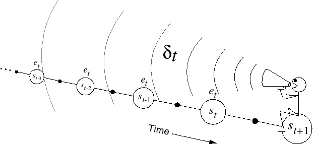
The TD error after each transition (s_t, a_t, r_{t+1}, s_{t+1}):
\delta_t = r_{t+1} + \gamma V(s_{t+1}) - V(s_t)
tells us how good the action a_t was compared to our expectation V(s_t).
When the advantage \delta_t > 0, this means that the action lead to a better reward or a better state than what was expected by V(s_t), which is a good surprise, so the action should be reinforced (selected again) and the value of that state increased. When \delta_t < 0, this means that the previous estimation of (s_t, a_t) was too high (bad surprise), so the action should be avoided in the future and the value of the state reduced.
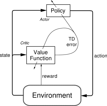
Actor-critic methods are TD methods that have a separate memory structure to explicitly represent the policy and the value function. The policy \pi is implemented by the actor, because it is used to select actions. The estimated values V(s) are implemented by the critic, because it criticizes the actions made by the actor.
The critic computes the TD error or 1-step advantage:
\delta_t = r_{t+1} + \gamma \, V(s_{t+1}) - V(s_t)
This scalar signal is the output of the critic and drives learning in both the actor and the critic. The critic is updated using this scalar signal:
V(s_t) \leftarrow V(s_t) + \alpha \, \delta_t
The actor is updated according to this TD error signal. For example a softmax actor over preferences:
\begin{cases} p(s_t, a_t) \leftarrow p(s_t, a_t) + \beta \, \delta_t \\ \\ \pi(s, a) = \frac{\exp{p(s, a)}}{\sum_b \exp{p(s, b)}} \\ \end{cases}
When \delta_t >0, the preference is increased, so the probability of selecting it again increases. When \delta_t <0, the preference is decreased, so the probability of selecting it again decreases.
The advantage of the separation between the actor and the critic is that now the actor can take any form (preferences, linear approximation, deep networks). It requires minimal computation in order to select the actions, in particular when the action space is huge or even continuous. It can learn stochastic policies, which is particularly useful in non-Markov problems.
However, it is obligatory to learn on-policy: the critic must evaluate the actions taken by the current actor, and the actor must learn from the current critic, not “old” V-values.
Classical TD learning only learn a value function (V^\pi(s) or Q^\pi(s, a)): these methods are called value-based methods. Actor-critic architectures are particularly important in policy search methods.
Advantage estimation
n-step advantages
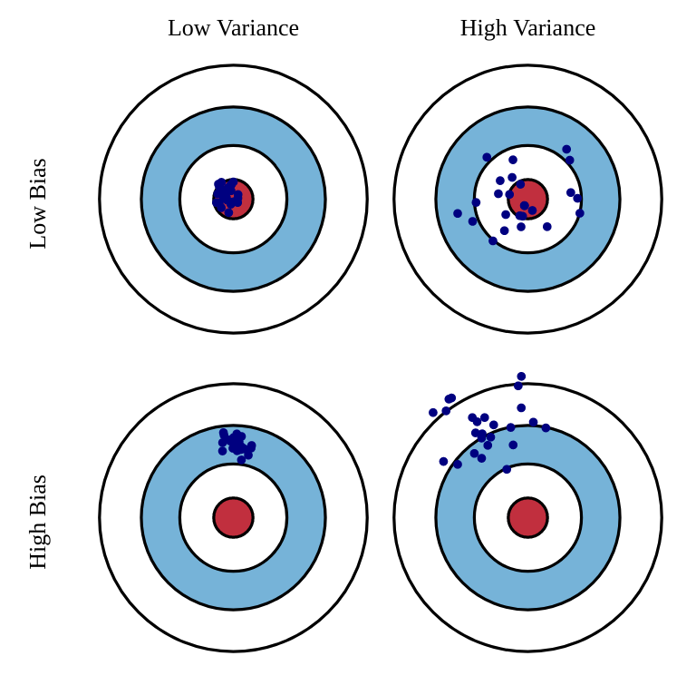
MC methods have high variance, low bias: Return estimates are correct on average, as we use real rewards from the environment, but each of them individually is wrong, because of the stochasticity of the policy/environment.
R_t^\text{MC} = \sum_{k=0}^{\infty} \gamma^k r_{t+k+1}
The small bias ensures good convergence properties, as we are more likely to find the optimal policy with correct estimates. The high variance means that we will need many samples to converge. The updates are not very sensitive to initial estimates.
On the other hand, TD has low variance, high bias, as the target returns contain mostly estimates.
R_t^\text{TD} = r_{t+1} + \gamma \, V^\pi(s_{t+1})
The only stochasticity comes from the immediate rewards, which is low, so the targets will not vary much during learning. But because they use other estimates, which are initially wrong, they will always be off. These wrong updates can, more often than not, lead to suboptimal policies. However, convergence will be much faster than with MC methods.
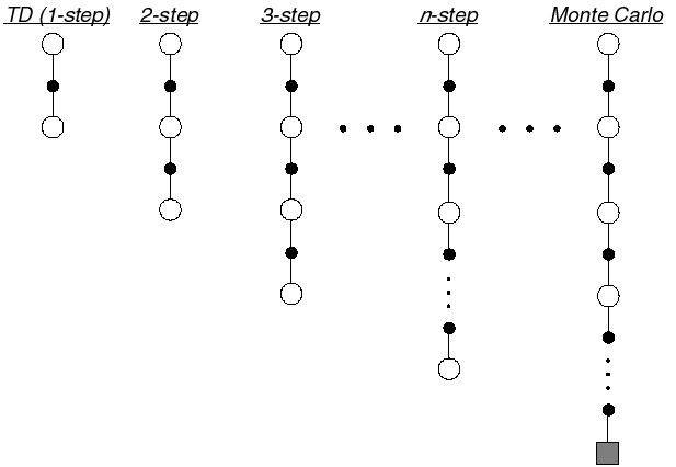
In order to control the bias-variance trade-off, we would like an estimator for the return with intermediate properties between MC and TD. This is what the n-step return offers:
R^n_t = \sum_{k=0}^{n-1} \gamma^{k} \, r_{t+k+1} + \gamma^n \, V(s_{t+n})
The n-step return uses the next n real rewards, and completes the rest of the sequence with the value of the state reached n steps in the future. Because it uses more real rewards than TD, its bias is smaller, while its variance is lower than MC.
The n-step advantage at time t is defined as the difference between the n-step return and the current estimate:
A^n_t = \sum_{k=0}^{n-1} \gamma^{k} \, r_{t+k+1} + \gamma^n \, V(s_{t+n}) - V (s_t)
It is easy to check that the TD error is the 1-step advantage:
\delta_t = A^1_t = r_{t+1} + \gamma \, V(s_{t+1}) - V(s_t)
n-step advantages are going to play an important role in deep RL, as the right choice of n will allow us to control the bias-variance trade-off: smaller values of n decrease the variance (smaller sample complexity) but may lead to suboptimal policies, while higher values of n converge to better policies, at the cost of necessitating more samples.
Eligibility traces
The main drawback of TD learning is that learning can be slow, especially when the problem provides sparse rewards (as opposed to dense rewards). For example in a game like chess, a reward is given only at the end of a game (+1 for winning, -1 for losing). All other actions receive a reward of 0, although they are as important as the last one in order to win.
Imagine you initialize all Q-values to 0 and apply Q-learning to the Gridworld problem of Figure 5.5. During the first episode, all actions but the last one will receive a reward of 0 and arrive in a state where the greedy action has a value Q^\pi(s', a') of 0 (initially), so the TD error \delta is 0 and their Q-value will not change. Only the very last action will receive a non-zero reward and update its value slightly (because of the learning rate \alpha).
When this episode is performed again, the last action will again be updated, but also the one just before: Q^\pi(s', a') is now different from 0 for this action, so the TD error is now different from 0. It is straightforward to see that if the episode has a length of 100 moves, the agent will need at least 100 episodes to “backpropagate” the final sparse reward to the first action of the episode. In practice, this is even worse: the learning rate \alpha and the discount rate \gamma will slow learning down even more. MC methods suffer less from this problem, as the first action of the episode would be updated using the actual return, which contains the final reward (although it is discounted by \gamma).
Eligibility traces can be seen a trick to mix the advantages of MC (faster updates) with the ones of TD (online learning, smaller variance). The idea is that the TD error at time t (\delta_t) will be used not only to update the action taken at time t (\Delta Q(s_t, a_t) = \alpha \, \delta_t), but also all the preceding actions, which are also responsible for the success or failure of the action taken at time t.
A parameter \lambda between 0 and 1 (decaying factor) controls how far back in time a single TD error influences past actions. This is important when the policy is mostly exploratory: initial actions may be mostly random and finally find the the reward by chance. They should learn less from the reward than the last one, otherwise they would be systematically reproduced. There are many possible implementations of eligibility traces (Watkin’s, Peng, Tree Backup, etc. See the Chapter 12 of Sutton and Barto (2017)). Generally, one distinguished a forward and a backward view of eligibility traces.
- The forward view considers that one transition (s_t, a_t) gathers the TD errors made at future time steps t' and discounts them with the parameter \lambda:
R_t^\lambda = \sum_{k=0}^T (\gamma \lambda)^{k} \delta_{t+k}
From this equation, \gamma and \lambda seem to play a relatively similar role, but remember that \gamma is also used inside the TD error, so they control different aspects of learning. The drawback of this approach is that the future transitions and their respective TD errors must be known when updating the transition, so this prevents online learning (the episode must be terminated to apply the updates, like in MC).
- The backward view considers that the TD error made at time t is sent backwards in time to all transitions previously executed. The easiest way to implement this is to update an eligibility trace e(s,a) for each possible transition, which is incremented every time a transition is visited and otherwise decays exponentially with a speed controlled by \lambda:
e(s, a) = \begin{cases} e(s, a) + 1 \quad \text{if} \quad s=s_t \quad \text{and} \quad a=a_t \\ \lambda \, e(s, a) \quad \text{otherwise.} \end{cases}
The Q-value of all transitions (s, a) (not only the one just executed) is then updated proportionally to the corresponding trace and the current TD error:
Q(s, a) \leftarrow Q(s, a) + \alpha \, e(s, a) \, \delta_{t} \quad \forall s, a
The forward and backward implementations are equivalent: the first requires to know the future, the second requires to update many transitions at each time step. The best solution will depend on the complexity of the problem.
TD learning, SARSA and Q-learning can all be efficiently extended using eligibility traces. This gives the algorithms TD(\lambda), SARSA(\lambda) and Q(\lambda), which can learn much faster than their 1-step equivalent, at the cost of more computations.
Generalized Advantage Estimation (GAE)
Let’s recall the n-step advantage:
A^{n}_t = \sum_{k=0}^{n-1} \gamma^{k} \, r_{t+k+1} + \gamma^n \, V^\pi(s_{t+n+1}) - V^\pi(s_t)
It is easy to show recursively that it depends on the TD error \delta_t = r_{t+1} + \gamma \, V^\pi(s_{t+1}) - V^\pi(s_t) of the n next steps:
A^{n}_t = \sum_{l=0}^{n-1} \gamma^l \, \delta_{t+l}
In other words, the prediction error over n steps is the (discounted) sum of the prediction errors between two successive steps. Now, what is the optimal value of n? GAE decides not to choose and to simply average all n-step advantages and to weight them with a discount parameter \lambda.
This defines the Generalized Advantage Estimator A^{\text{GAE}(\gamma, \lambda)}_t:
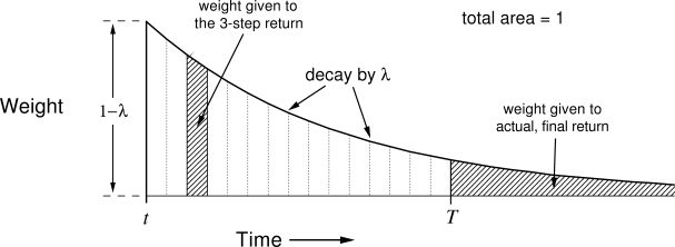
A^{\text{GAE}(\gamma, \lambda)}_t = (1-\lambda) \, \sum_{l=0}^\infty \lambda^l A^l_t = \sum_{l=0}^\infty (\gamma \lambda)^l \delta_{t+l}
The GAE is simply a forward eligibility trace over distant n-step advantages: the 1-step advantage is more important the the 1000-step advantage (too much variance).
- When \lambda=0, we have A^{\text{GAE}(\gamma, 0)}_t = A^{0}_t = \delta_t, i.e. the TD advantage (high bias, low variance).
- When \lambda=1, we have (at the limit) A^{\text{GAE}(\gamma, 1)}_t = R_t, i.e. the MC advantage (low bias, high variance).
Choosing the right value of \lambda between 0 and 1 allows to control the bias/variance trade-off.
\gamma and \lambda play different roles in GAE: \gamma determines the scale or horizon of the value functions: how much future rewards rewards are to be taken into account. The higher \gamma <1, the smaller the bias, but the higher the variance. Empirically, Schulman et al. (2015) found that small \lambda values introduce less bias than \gamma, so \lambda can be chosen smaller than \gamma (which is typically 0.99).
In practice, GAE leads to a better estimation than n-step advantages, but is more computationally expensive. It is used in particular in PPO (Section Proximal Policy Optimization (PPO)).

