Planning (MPC, TDM)

Model-based learning is not only used to augment MF methods with imaginary rollouts. It can also be use directly for planning, as the model s', r = M(s, a) can emulate complete trajectories and estimate their return.

s_0 \xrightarrow[\pi]{} a_0 \xrightarrow[M]{} s_1 \xrightarrow[\pi]{} a_1 \xrightarrow[\pi]{} s_2 \xrightarrow[]{} \ldots \xrightarrow[M]{} s_T

A non-linear optimization procedure can then learn to select a policy that maximizes the return. It can either be:

• Model-free RL methods,
• Classical non-linear optimization methods such as iLQR (Iterative Linear Quadratic Regulator, see https://jonathan-hui.medium.com/rl-lqr-ilqr-linear-quadratic-regulator-a5de5104c750 for explanations).
• Stochastic sampling methods such as the cross-entropy method CEM, where the policy is randomly sampled and improved over successive rollouts (Szita and Lörincz, 2006),
• Genetic algorithms such as Evolutionary Search (ES) (Salimans et al., 2017).

For long horizons, the slightest imperfection in the model can accumulate over time (drift) and lead to completely wrong trajectories.

Figure 22.1: Planning over long trajectories can accumulate imperfections in the model. Source: https://medium.com/@jonathan_hui/rl-model-based-reinforcement-learning-3c2b6f0aa323

The emulated trajectories will have a biased return, and the optimization algorithm will not converge to the optimal policy. If you have a perfect model at your disposal, you should not be using RL anyway, as classical control methods would be much faster in principle (but see AlphaGo).

Model Predictive Control

The solution is to replan at each time step and execute only the first planned action in the real environment. After this step is performed, we plan again.

Figure 22.2: Replanning after each step allows to compensate for model errors. Source: https://medium.com/@jonathan_hui/rl-model-based-reinforcement-learning-3c2b6f0aa323

Model Predictive Control iteratively plans complete trajectories, but only selects the first action. This can be computationally expensive, but prediction errors do not accumulate.

Model Predictive Control

• Collect transitions (s, a, r, s') using a (random/expert) policy b and create an initial dataset \mathcal{D} = \{(s_k, a_k, r_, s'_k\}_{k}.

• while not converged:

  • (Re)Train the dynamics model M(s, a) = (s', r) on \mathcal{D} using supervised learning.

  • foreach step t in the trajectory:

    • Plan a trajectory from the current state s_t using the model M, returning a sequence of planned actions:

    a_{t}, a_{t+1}, \ldots, a_T

    • Take the first action a_t, observe the next state s_{t+1}.

    • Append the transition (s_t, a_t, s_{t+1}) to the dataset.

The frequency at which the dynamics model is retrained or fine-tune may vary from implementation to implementation, it does not have to be between each trajectory. See http://rail.eecs.berkeley.edu/deeprlcourse-fa17/f17docs/lecture_9_model_based_rl.pdf for more details on MPC.

Example with a neural dynamics model

Model-predictive control using a learned model. Source: Nagabandi et al. (2017).

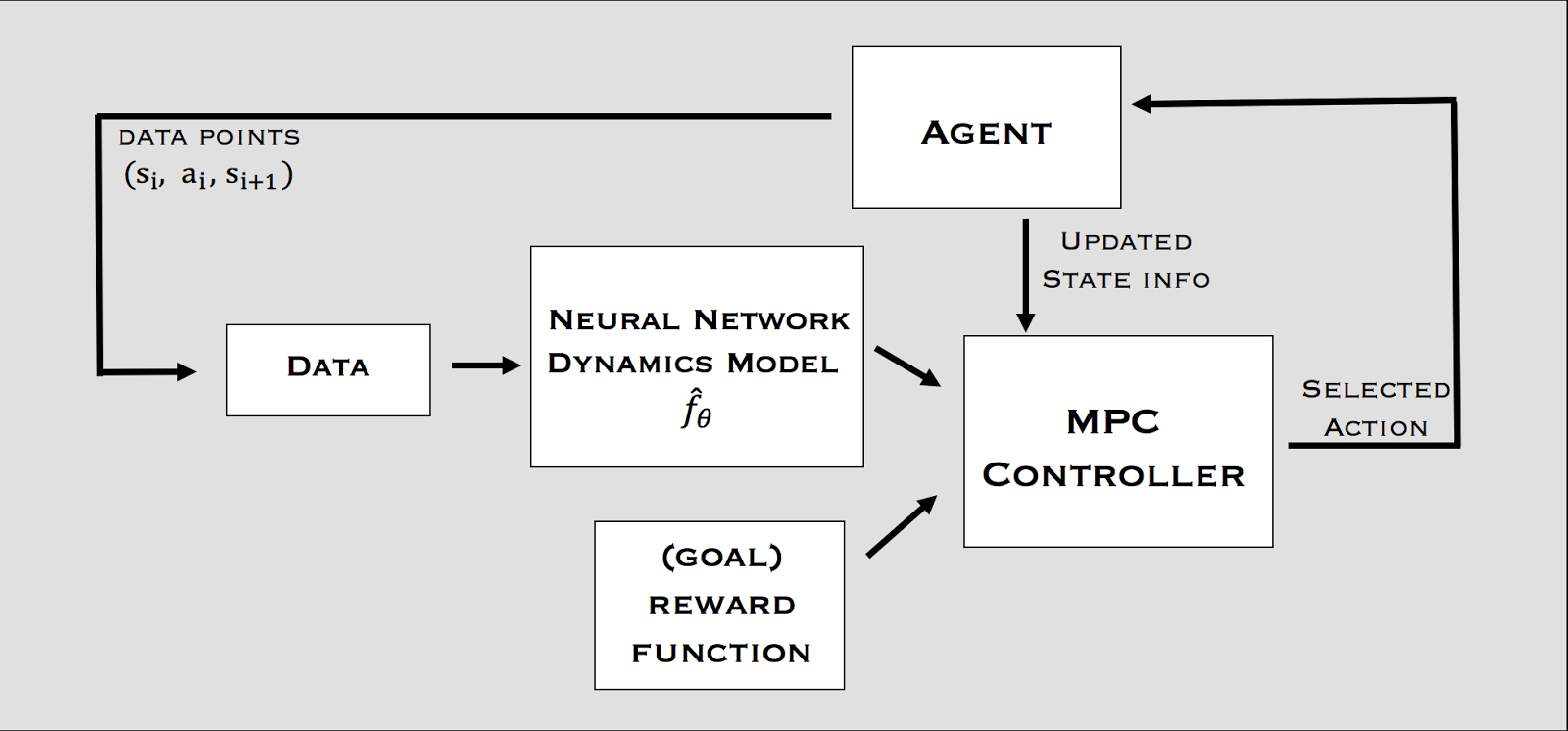
In Nagabandi et al. (2017), the dynamics model is a neural network predicting the next state and the associated reward. The controller uses random-sampling shooting:

1. In the current state, a set of possible actions is selected.
2. Rollouts are generated from these actions using the model and their return is computed.
3. The initial action of the rollout with the highest return is selected.
4. Repeat.

Figure 22.3: Random-sampling shooting. Using different initial actions, several imaginary rollouts are performed. The one leading to the maximal return is chosen and executed. Source: https://bair.berkeley.edu/blog/2017/11/30/model-based-rl/

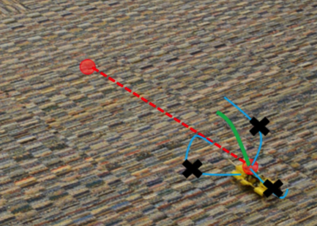
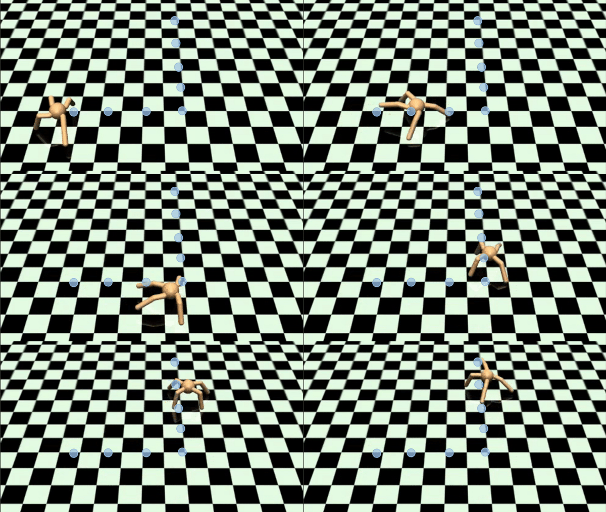
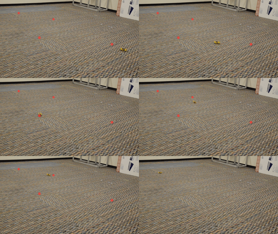
The main advantage of MPC is that you can change the reward function (the goal) on the fly: what you learn is the model, but planning is just an optimization procedure. You can set intermediary goals to the agent very flexibly: no need for a well-defined reward function. Model imperfection is not a problem as you replan all the time. As seen below, the model can adapt to changes in the environment (slippery terrain, simulation to real-world).

Figure 22.4: Source: https://bair.berkeley.edu/blog/2017/11/30/model-based-rl/

Figure 22.5: Source: https://bair.berkeley.edu/blog/2017/11/30/model-based-rl/

Temporal difference models - TDM

Planning over long horizon

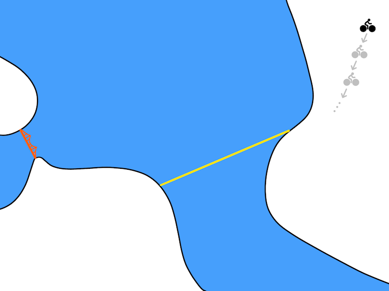
One problem with model-based planning is the discretization time step (difference between t and t+1). It is determined by the action rate: how often a different action a_t has to be taken. In robotics, it could be below the millisecond, leading to very long trajectories in terms of steps.

Figure 22.6: Example of going from Berkeley to the Golden Gate bridge with a bike. Source: Pong et al. (2018) and https://bairblog.github.io/2018/04/26/tdm/

If you want to go from Berkeley to the Golden Gate bridge with your bike, planning over leg movements will be very expensive (long horizon). A solution is to use multiple steps ahead planning. Instead of learning a one-step model:

s_{t+1} = f_\theta(s_t, a_t)

one learns to predict the state achieved in T steps using the current policy:

s_{t+ T} = f_\theta(s_t, a_t, \pi)

Planning and acting can occur at different time scales: as in MPC, you plan for a significant number of steps in the future, but you only take the first step. If you learn to predict directly T steps into the future, you do not even need the intermediary steps.

Goal-conditioned RL

Another problem with RL in general is how to define the reward function. If you goal is to travel from Berkeley to the Golden State bridge, which reward function should you use?

• +1 at the bridge, 0 otherwise (sparse).
• +100 at the bridge, -1 otherwise (sparse).
• minus the distance to the bridge (dense).

Moreover, do you have to re-learn everything if you want to go somewhere else?

Goal-conditioned RL defines the reward function using the distance between the achieved state s_{t+1} and a goal state s_g:

r(s_t, a_t, s_{t+1}) = - || s_{t+1} - s_g ||

An action will reinforced if it brings the agent closer to its goal. The Euclidean distance works well for the biking example (e.g. using a GPS), but the metric can be adapted to the task. One advantage is that you can learn multiple “tasks” at the same time with a single policy, not the only one hard-coded in the reward function.

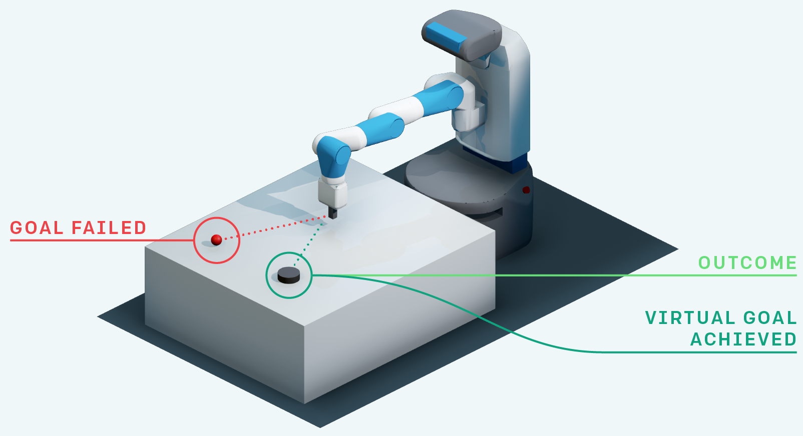
Another advantage is that it makes a better use of exploration by learning from mistakes, as in hindsight experience replay (HER, Andrychowicz et al. (2017)). If your goal is to reach s_g but the agent generates a trajectory landing in s_{g'}, you can learn that this trajectory is a good way to reach s_{g'}! In football, if you try to score a goal but end up doing a pass to a teammate, you can learn that this was a bad shot and a good pass. HER is a model-based method: you implicitly learn a model of the environment by knowing how to reach any position.

Figure 22.7: Hindsight experience replay. Source: https://openai.com/blog/ingredients-for-robotics-research/

Exploration never fails: you always learn to do something, even if this was not your original goal. The principle of HER can be combined with all model-free methods: DQN, DDPG, etc. Your value / policy network only has to take inputs from s and g instead of only s.

TDM

Using the goal-conditioned reward function r(s_t, a_t, s_{t+1}) = - || s_{t+1} - s_g ||, how can we learn? TDM (Pong et al., 2018) introduces goal-conditioned Q-values with a horizon T: Q(s, a, s_g, T). The Q-value of an action should denote how close we will be from the goal s_g in T steps. If we can estimate these Q-values, we can use a planning algorithm such as MPC to find the action that will bring us closer to the goal easily:

a^* = \text{arg}\max_{a_t} \, r(s_{t+T}, a_{t+T}, s_{t+T + 1})

This corresponds to planning T steps ahead: which action should I do now in order to be close to the goal in T steps? If the horizon T is well chosen, we only need to plan over a small number of intermediary positions, not over each possible action. TDM is model-free on each subgoal, but model-based on the whole trajectory.

How can we learn the goal-conditioned Q-values Q(s, a, s_g, T) with a model? TDM introduces a recursive relationship for the Q-values:

\begin{aligned} Q(s, a, s_g, T) &= \begin{cases} \mathbb{E}_{s'} [r(s, a, s')] \; \text{if} \; T=0\\ &\\ \mathbb{E}_{s'} [\max_a \, Q(s', a, s_g, T-1)] \; \text{otherwise.}\\ \end{cases} \\ &\\ &= \mathbb{E}_{s'} [r(s, a, s') \, \mathbb{1}(T=0) + \max_a \, Q(s', a, s_g, T-1) \, \mathbb{1}(T\neq 0)]\\ \end{aligned}

If we plan over T=0 steps, i.e. immediately after the action (s, a), the Q-value is the remaining distance to the goal from the next state s'. Otherwise, it is the Q-value of the greedy action in the next state s' with an horizon T-1 (one step shorter). This allows to learn the Q-values from single transitions (s_t, a_t, s_{t+1}):

• with T=0, the target is the remaining distance to the goal.
• with T>0, the target is the Q-value of the next action at a shorter horizon.

The critic learns to minimize the prediction error off-policy:

\begin{aligned} \mathcal{L}(\theta) = & \mathbb{E}_{s_t, a_t, s_{t+1} \in \mathcal{D}} [ & \\ & (r(s_t, a_t, s_{t+1}) \, \mathbb{1}(T=0) + \max_a \, Q(s_{t+1}, a, s_g, T-1) \, \mathbb{1}(T\neq 0) - Q(s_t, a_t, s_g, T))^2 & \\ && ] \end{aligned}

This is a model-free Q-learning-like update rule, that can be learned by any off-policy value-based algorithm (DQN, DDPG) and an experience replay memory. The cool trick is that, with a single transition (s_t, a_t, s_{t+1}), you can train the critic with:

• different horizons T, e.g. between 0 and T_\text{max}.
• different goals s_g. You can sample any achievable state as a goal, including the “true” s_{t+T} (hindsight).

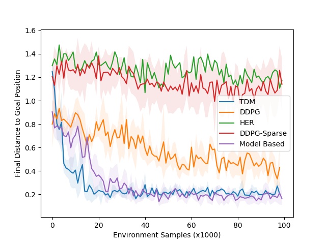
You do not only learn to reach s_g, but any state! TDM learns a lot of information from a single transition, so it has a very good sample complexity. TDM learns to break long trajectories into finite horizons (model-based planning) by learning model-free (Q-learning) updates. TDM is a model-based method in disguise: it does predict the next state directly, but how much closer it will be to the goal via Q-learning.

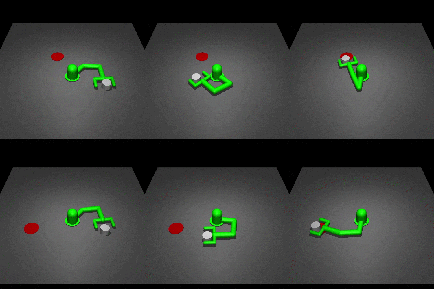
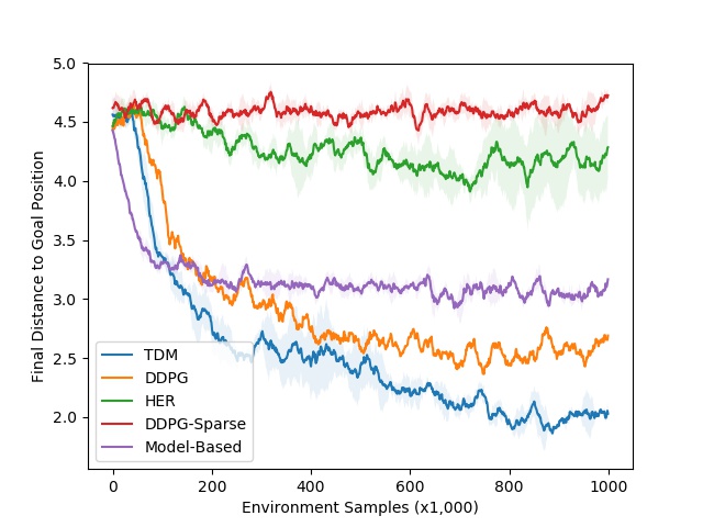
For problems where the model is easy to learn, the performance of TDM is on par with model-based methods (MPC).

Source: https://bairblog.github.io/2018/04/26/tdm/

Model-free methods have a much higher sample complexity, while TDM learns much more from single transitions.

Source: https://bairblog.github.io/2018/04/26/tdm/

For problems where the model is complex to learn, the performance of TDM is on par with model-free methods (DDPG).

Source: https://bairblog.github.io/2018/04/26/tdm/

Model-based methods suffer from model imprecision on long horizons, while TDM plans over shorter horizons T.

Source: https://bairblog.github.io/2018/04/26/tdm/

Andrychowicz, M., Wolski, F., Ray, A., Schneider, J., Fong, R., Welinder, P., et al. (2017). Hindsight Experience Replay. Available at: http://arxiv.org/abs/1707.01495.

Nagabandi, A., Kahn, G., Fearing, R. S., and Levine, S. (2017). Neural Network Dynamics for Model-Based Deep Reinforcement Learning with Model-Free Fine-Tuning. Available at: http://arxiv.org/abs/1708.02596 [Accessed March 3, 2019].

Pong, V., Gu, S., Dalal, M., and Levine, S. (2018). Temporal Difference Models: Model-Free Deep RL for Model-Based Control. Available at: http://arxiv.org/abs/1802.09081.

Salimans, T., Ho, J., Chen, X., Sidor, S., and Sutskever, I. (2017). Evolution Strategies as a Scalable Alternative to Reinforcement Learning. Available at: http://arxiv.org/abs/1703.03864.

Szita, I., and Lörincz, A. (2006). Learning Tetris Using the Noisy Cross-Entropy Method. Neural Computation 18, 2936–2941. doi:10.1162/neco.2006.18.12.2936.