Intrinsic motivation
All the methods presented in this book depend entirely on the reward function. The agent maximizes the returns, so whatever we put in the reward function is what we get. This is fine as long as we are able to write down a reward function that describes what we want, and as long as the agent is able to collect some reward by exploring randomly at the beginning of learning. Both assumptions are problematic.
The problem with sparse rewards
Let’s start with the second assumption. With sparse rewards (Monte Carlo methods), the agent only receives a non-zero reward in a few rare transitions: winning the game, reaching the goal, grasping the object. Everywhere else, the reward is 0.
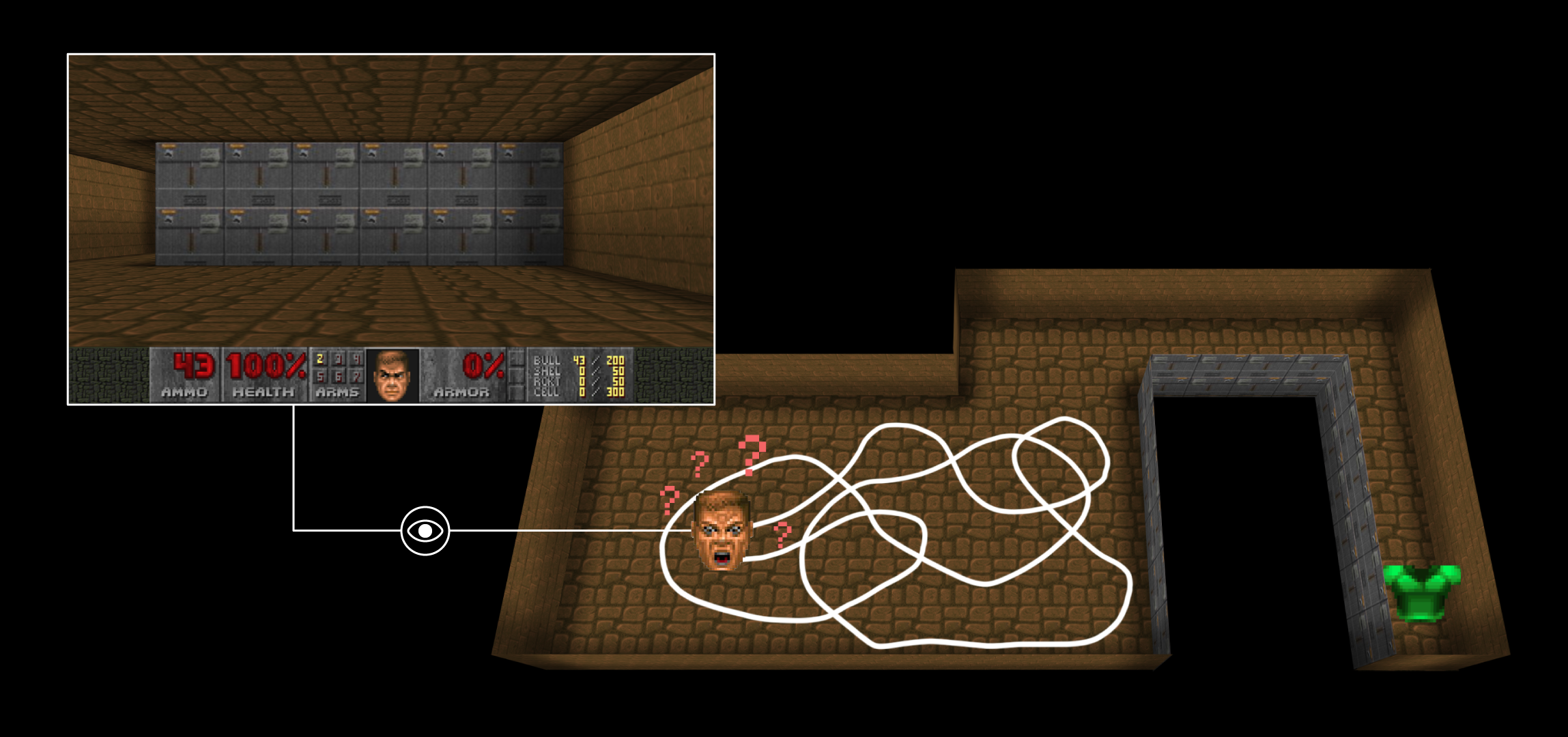
Before the agent stumbles on a reward by chance, all the transitions it experiences have a reward of 0 and all its value estimates stay at 0, so the TD error is 0 and nothing is learned. The agent does not become “better at exploring” during that phase: it is a random agent, and it stays a random agent until the first reward arrives. If the reward is far away, the probability of reaching it by executing random actions decreases exponentially with the distance.
This is exactly what happened to DQN on Montezuma’s Revenge (Deep Q-network (DQN)). In this Atari game, the agent must climb down a ladder, jump over a skull, pick up a key, come back, and open a door. Only then does it receive a reward. A random agent essentially never completes that sequence, so DQN scored 0 on the game while reaching super-human performance on most of the others. Adding more layers or more training time does not help: the problem is not the capacity of the network, it is that the reward signal never arrives.
The first assumption is not much better. Writing the “right” reward function is an art, and a badly designed one leads to an agent that maximizes exactly what you asked for instead of what you wanted (we will come back to that in Inverse Reinforcement Learning). In many realistic problems, we may not even be able to say what the reward should be.
So the question of this chapter is:
can the agent generate its own reward signal, in order to learn something useful even when the environment does not tell it anything?
Intrinsic motivation
The inspiration comes again from animal behavior. Humans, and especially infants, do not spend their time maximizing external rewards. They play: they push objects off the table, they open and close doors, they babble. None of this brings any food or any grade. They do it because it is interesting.
Psychologists call this intrinsic motivation: a behavior done for its own sake, as opposed to extrinsic motivation, a behavior done to obtain an external reward (Barto, 2013). The useful thing about playing is that it builds a model of the world, which becomes extremely valuable later, when there finally is a goal to achieve.
The idea in RL is to give the agent an additional reward that it computes by itself, the intrinsic reward r^i_t, and to have it maximize the sum of both:
r_t = r^e_t + \beta \, r^i_t
where r^e_t is the usual extrinsic reward coming from the environment, and \beta weights how curious the agent should be.
One may wonder whether this is not cheating. If the agent produces its own rewards, what prevents it from simply giving itself an infinite reward and stopping there? Barto (2013) proposes a useful way to think about it, depicted on Figure 24.2. What we usually call the environment in the agent-environment interface is in fact the external environment. The reward signal is not produced by it, but by a critic which belongs to the internal environment of the organism. Both the critic and the RL agent are inside the organism, but the RL agent does not control the critic: from its point of view, the reward is still something that it receives, not something that it chooses.
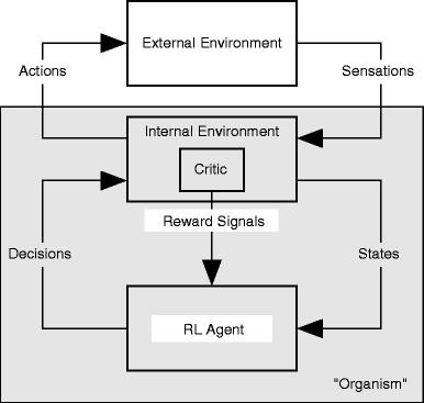
In this view, extrinsic and intrinsic rewards are not different in nature: they are both produced by the same internal critic. What differs is only what triggers them, an event in the external environment or an event inside the organism. Hunger, curiosity or boredom are as “real” as a reward given by a teacher.
Note that this changes nothing to the algorithms themselves: we can use DQN, A3C, PPO or SAC without any modification, we only modify the reward that we feed them. This is why intrinsic motivation is so widely used: it is a module that can be plugged on top of any RL algorithm.
The idea is not new: Schmidhuber (2010) had been formalizing it since 1990, under the names of curiosity, fun and creativity. His formulation is worth remembering, because it is subtly different from what most modern methods do: the intrinsic reward should not be the error of the agent’s model, but the improvement of that model, i.e. the learning progress. Rewarding the error pushes the agent towards what it cannot predict; rewarding the progress pushes it towards what it is currently able to learn. We will see very soon why this distinction matters.
The whole difficulty is now to define r^i_t: what should be intrinsically rewarding?
Curiosity as a prediction error
A reasonable answer is: what is surprising. If you can perfectly predict what is going to happen, the situation is boring and there is nothing to learn from it. If you cannot predict what happens, you have found a part of the world that your model does not cover yet, and it is worth exploring.
This can be measured directly. Let’s learn a forward model f that predicts the next state from the current state and action, exactly as in model-based RL (World models, Dreamer):
\hat{s}_{t+1} = f(s_t, a_t)
and define the intrinsic reward as the error made by this prediction:
r^i_t = || f(s_t, a_t) - s_{t+1} ||^2
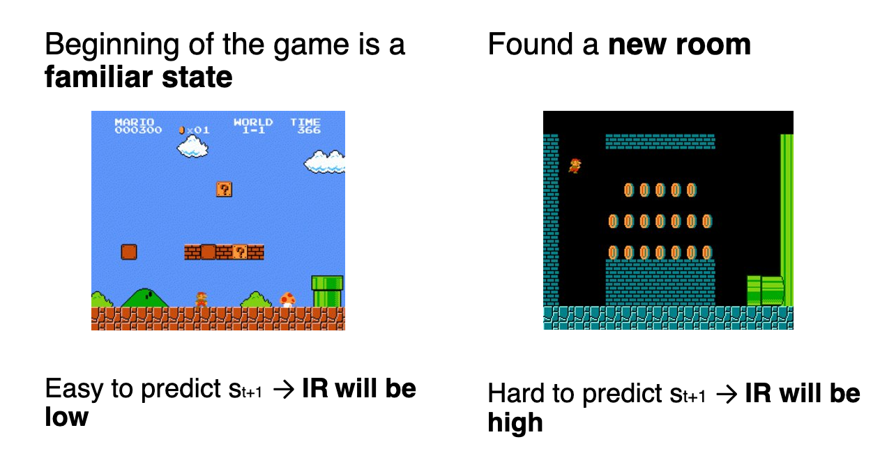
An agent maximizing this reward will systematically go towards the transitions that its model predicts badly, i.e. the parts of the environment it does not know yet. This is exploration, but a directed one: instead of taking random actions and hoping, the agent actively seeks novelty.
A very nice property of this scheme is that it is self-limiting. The forward model is trained on the transitions that the agent experiences, so the more often the agent visits a region, the better the model predicts it, and the smaller the intrinsic reward becomes. Curiosity therefore extinguishes itself in regions that have been understood, and the agent moves on. Compare this to \epsilon-greedy, where the exploration level is a hyperparameter that we have to schedule by hand and which is the same everywhere in the state space.
The noisy-TV problem
Unfortunately, computing the prediction error directly on the states does not work well.
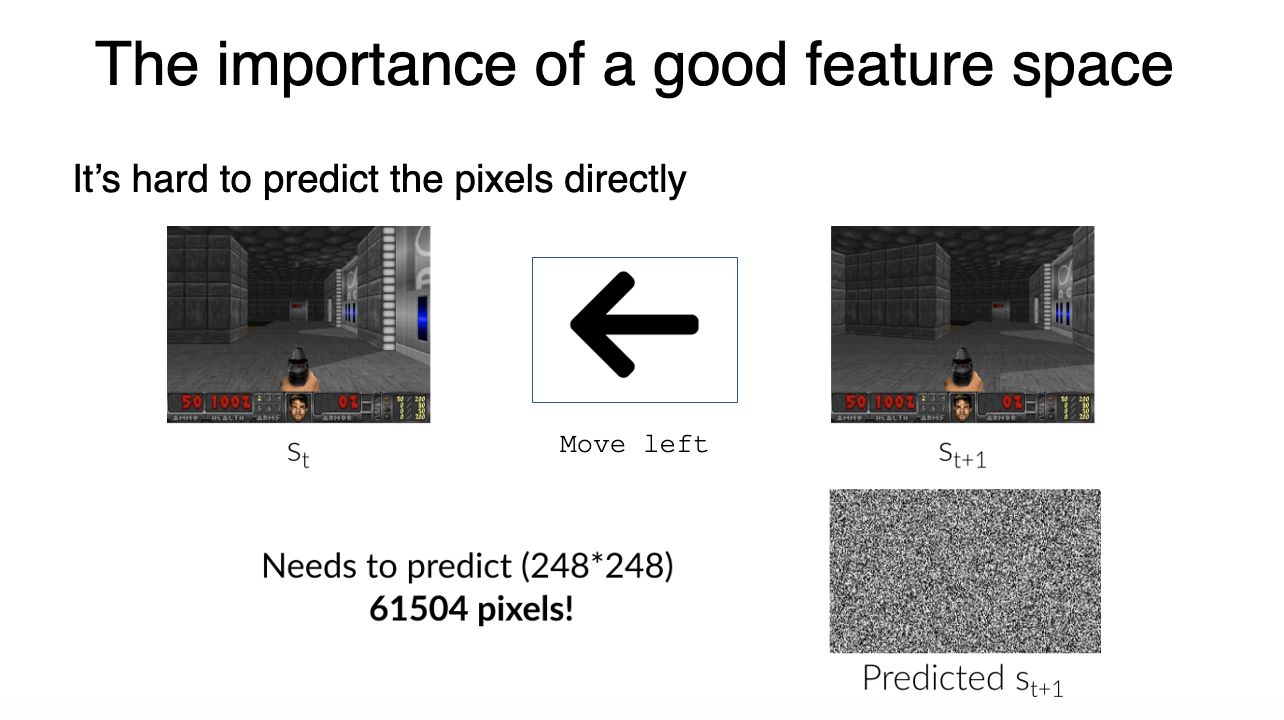
The first issue is technical: when the states are images, predicting the next frame means predicting tens of thousands of pixels. This is a hard problem in itself, and the prediction will never be perfect, so there will always be a residual error and therefore a residual intrinsic reward everywhere.
The second issue is much more fundamental. Some things in the world are unpredictable but not interesting: leaves moving in the wind, noise on a screen, the result of a dice throw. The prediction error on those will stay high forever, because the randomness is irreducible: no amount of learning will let you predict which way a leaf moves next.

An agent maximizing the prediction error will happily park itself in front of such a source of noise and collect a large intrinsic reward forever, without learning anything and without exploring anything else. This failure mode is known as the noisy-TV problem: put a TV showing static in a maze, and your curious agent will stop exploring the maze and watch the TV.
Note that this is the exact opposite of what we wanted: we introduced curiosity to make exploration smarter, and we ended up with an agent that gets addicted to noise. This is also exactly the distinction made by Schmidhuber (2010): in front of the noisy TV, the prediction error stays maximal forever, but the learning progress is zero, as the model does not improve at all. An agent rewarded by its progress would lose interest immediately. Measuring progress is unfortunately much harder than measuring error, so most practical methods keep the error and try to fix the problem another way: by being more careful about what the agent tries to predict.
Intrinsic Curiosity Module (ICM)
The Intrinsic Curiosity Module (ICM, Pathak et al., 2017) solves both issues at once with a simple idea: do not predict the next state, predict a learned representation of the next state, and learn that representation so that it only contains what the agent can influence.
The ICM has three components:
- A feature encoder \phi, which maps a state s_t to a feature vector \phi(s_t) of much smaller dimensionality.
- A forward model, which predicts the features of the next state from the features of the current state and the action: \hat{\phi}(s_{t+1}) = f(\phi(s_t), a_t)
- An inverse model, which predicts which action was taken between two successive states: \hat{a}_t = g(\phi(s_t), \phi(s_{t+1}))
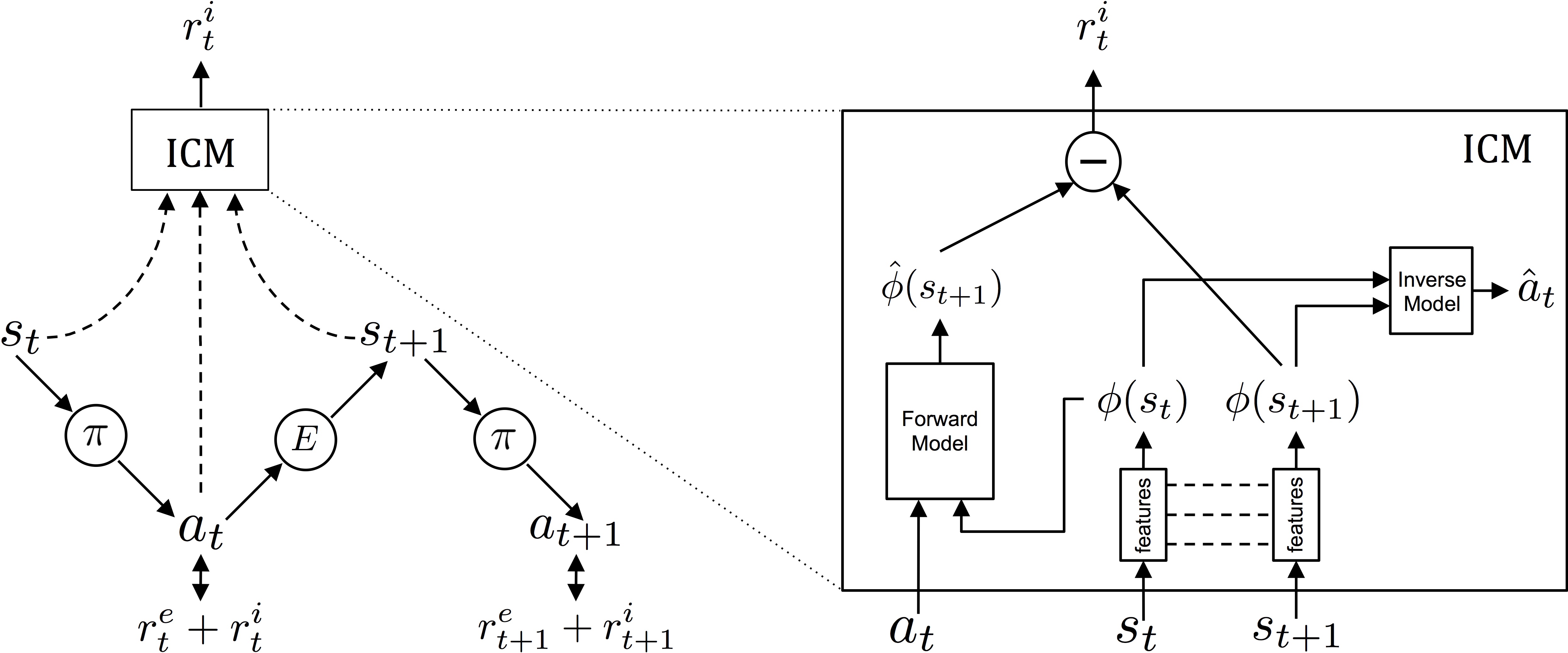
The intrinsic reward is now the prediction error of the forward model in the feature space:
r^i_t = || \hat{\phi}(s_{t+1}) - \phi(s_{t+1}) ||^2
which is a much smaller and easier prediction problem than working on raw pixels.
But the real trick is the inverse model. The encoder \phi is not trained to reconstruct the states (as an autoencoder would), it is trained so that the inverse model can recover the action. Think about what this implies:
- If some part of the observation is influenced by the agent’s actions (the position of its own body, the objects it pushes), it is useful to predict the action, so \phi keeps it.
- If some part of the observation is not influenced by the agent at all (the leaves in the wind, the TV static, the clouds in the background), it is useless to predict the action, so \phi learns to discard it.
The feature space therefore only encodes the part of the environment that the agent can control or that affects it, and the noisy-TV disappears from the representation before the intrinsic reward is even computed. This is an elegant solution, and it is worth remembering as a general principle: when a quantity is hard to define directly, one can often define an auxiliary task whose solution forces the right quantity to emerge.
ICM allows agents to learn to play games such as VizDoom and Super Mario Bros with very sparse rewards, and even with no extrinsic reward at all.
Burda et al. (2018a) later performed a large-scale study of purely curiosity-driven learning, i.e. with the extrinsic reward completely removed (r_t = r^i_t), on 54 benchmark environments including the whole Atari suite. The results are surprising: on many games, an agent that has never seen a single point of game score still learns to play reasonably well. The explanation is that these games are designed by humans for humans, so the game score is usually well aligned with “making interesting things happen on the screen” — progressing in the level is exactly what a curious agent wants to do anyway.
Counting states
Let’s take a step back. All the methods above measure surprise: how badly does my model predict what is going to happen? But what we actually want for exploration is novelty: have I been here before? The two are related, as a state which has never been visited is usually predicted badly, but they are not the same thing, and the noisy TV is precisely a case where a state stays surprising forever while not being novel at all.
If novelty is what we want, why not measure it directly? In tabular RL, this is trivial: keep a counter N(s) of the number of times each state has been visited, and give a bonus that decreases with it, for example:
r^i_t = \frac{1}{\sqrt{N(s_t)}}
This is a very old idea, and in the tabular case it can even be proven to lead to near-optimal exploration. The problem is that it does not survive the passage to deep RL. When the states are images, no two frames are ever identical pixel by pixel, so every state is visited exactly once, all counts are 1, and the bonus is the same everywhere: useless. Counting requires the states to be discrete and to repeat, which is exactly the assumption that function approximation was introduced to get rid of (Function approximation).
Bellemare et al. (2016) found an elegant way around this, called pseudo-counts. The idea is to replace the counter by a density model \rho(s), i.e. a model that estimates the probability of observing the state s, and which is trained on the states that the agent visits. Contrary to a counter, a density model generalizes: a state which resembles many already visited states receives a high probability, even if this exact state has never been seen.
The question is then how to get a count back out of a probability. Let’s note \rho(s) the probability that the model assigns to s, and \rho'(s) the probability that it would assign to s after being trained on s one more time. If the density model behaved exactly like a counter having seen n states in total, we would have:
\rho(s) = \frac{N(s)}{n} \qquad \qquad \rho'(s) = \frac{N(s) + 1}{n + 1}
These are two equations with two unknowns (N(s) and n), so we can solve them for N(s) and obtain the pseudo-count:
\hat{N}(s) = \frac{\rho(s) \, (1 - \rho'(s))}{\rho'(s) - \rho(s)}
which can now be computed for any density model and used in the exploration bonus in place of the true count. Said differently: how much the model improves when forced to learn a state one more time tells us how many times it has effectively already seen it. A state the model already knows well barely changes, so \rho'(s) \approx \rho(s), the denominator is tiny and the pseudo-count is huge. A completely new state changes the model a lot, and the pseudo-count is small.
It is worth noticing that this is precisely Schmidhuber (2010)’s learning progress, measured on a density model instead of a forward model. Pseudo-counts are therefore immune to the noisy TV for the same reason: watching static does not improve the density model, so the pseudo-count stops growing and the bonus vanishes.
Applied to Atari with a simple pixel density model, pseudo-counts produced the first real progress on Montezuma’s Revenge. Ostrovski et al. (2017) then replaced the density model by PixelCNN, a much better neural density model for images, and improved the results further, confirming that the quality of the density model directly determines the quality of the exploration.
Random Network Distillation (RND)
Pseudo-counts work, but they require training a density model over images, which is heavy and delicate: the whole scheme depends on the density model being well calibrated, and image density models are hard to get right.
Random Network Distillation (RND, Burda et al., 2018b) obtains a very similar notion of novelty far more cheaply, with a trick that looks like a joke at first sight. Take two networks:
- A target network \hat{f} with random weights, which is fixed and never trained.
- A predictor network f_\psi, which is trained to predict the output of the target network on the states that the agent visits, by minimizing:
\mathcal{L}(\psi) = || f_\psi(s_t) - \hat{f}(s_t) ||^2
The intrinsic reward is simply this prediction error:
r^i_t = || f_\psi(s_t) - \hat{f}(s_t) ||^2
Why does this work? The function to be predicted is now deterministic by construction: \hat{f} is a fixed function of the state, it contains no noise whatsoever. There is therefore no irreducible error: on a state that has been visited often, the predictor can in principle become perfect and the intrinsic reward goes to 0. On a state that has never been visited, the predictor has no reason to be correct and the error is high.
The prediction error has stopped measuring “how unpredictable is the future” and now measures “how novel is this state”, which is what we wanted in the first place. A stochastic TV does not fool RND: whatever the screen shows, \hat{f} maps it to a fixed output, and once the predictor has seen enough screens it predicts them all.
RND is also trivial to implement (two small networks and one mse loss, no forward model, no inverse model, no density model) and adds almost no computation. Combined with PPO, it established the state of the art on Montezuma’s Revenge and was the first method to exceed average human performance on it, five years after DQN had scored zero on the same game.
Episodic curiosity
Pseudo-counts and RND both measure novelty with respect to everything the agent has seen since the beginning of training. Savinov et al. (2019) propose a different and quite intuitive notion: novelty with respect to the current episode, measured in number of steps.
The agent maintains an episodic memory containing the observations encountered since the beginning of the episode. A network is trained to predict, for a pair of observations, whether one is reachable from the other within k steps. The intrinsic reward of the current observation is then high if it is far, in number of steps, from everything already in memory, and low if it can be reached quickly from something already seen. At the end of the episode, the memory is emptied.
The interesting point is that this measure is about the dynamics of the environment, not about the appearance of the states. Turning on the spot produces a continuous stream of very different images, so any appearance-based novelty measure rewards it. But all these images are reachable from one another in one or two steps, so reachability-based curiosity does not reward it at all. The noisy TV is defeated once more, this time by asking a question about the structure of the environment rather than about the pixels.
Planning to explore
All the methods above are retrospective: the agent computes the novelty of a state after having reached it. It discovers that a region was interesting only once it is already there, which is still a form of trial and error.
If we have a world model (World models, Dreamer), we can do better and seek out novelty before experiencing it. This is the idea of Plan2Explore (Sekar et al., 2020), which builds on Dreamer. Instead of a single forward model, it trains an ensemble of forward models in the latent space. On a part of the environment that has been seen often, all the models agree with each other. On a part that has not, they disagree, because each of them extrapolates differently.
The disagreement between the models (the variance of their predictions) is therefore a measure of novelty that can be computed in imagination, without acting. The agent can then plan a trajectory towards the states where the ensemble expects to disagree, i.e. actively navigate towards what it does not know yet.
The consequence is that the agent explores with no task and no reward at all, purely building a world model, and afterwards it can solve new tasks that were not known during exploration, sometimes in a zero-shot manner: once the world model is good, a new reward function is all that is needed to derive a new behavior by planning in imagination.
This closes a nice loop with World models, Dreamer: a world model makes better exploration possible, and better exploration makes a better world model.
Is novelty enough?
All the methods presented so far follow the same recipe: define a measure of novelty, turn it into a reward, and let a standard RL algorithm maximize it. Ecoffet et al. (2021) argue that this recipe has a structural weakness, and that this weakness, rather than the quality of the novelty measure, is what really limits exploration. They identify two failure modes:
- Detachment: the agent discovers a promising area and starts exploring it, but its policy drifts elsewhere in the meantime. When it comes back, the states of that area are not novel anymore, so their intrinsic reward has already been consumed and there is nothing left to attract the agent. It has effectively forgotten that there was something to explore there.
- Derailment: even when the agent does know that a distant state is worth exploring from, it has to travel back to it using its own stochastic, exploratory policy. The longer the path, the more likely the exploratory noise makes it fail somewhere on the way. The very randomness that is needed to explore prevents the agent from reaching the place where it should explore.
Their algorithm, Go-Explore, gives up on the intrinsic reward entirely. It keeps instead an explicit archive of the interesting states that have been reached, together with a trajectory leading to each of them, and repeats the two steps which give the paper its title:
- First return: select a promising state from the archive and go back to it directly, by replaying the stored trajectory (or, in the stochastic case, by training a policy to imitate it), rather than by exploring.
- Then explore: from there, explore randomly, and add every newly discovered state to the archive.
Separating “coming back” from “exploring” removes both failure modes at once: nothing is forgotten, because the archive is explicit and permanent, and nothing is derailed, because returning does not rely on a noisy policy. Go-Explore solved Montezuma’s Revenge outright, above the human world record, and scored above the state of the art on all the hard-exploration Atari games.
This is a useful result to keep in mind, because it says something slightly uncomfortable about the rest of this chapter. The hard part of exploration may not be estimating novelty, which is what ICM, pseudo-counts, RND and episodic curiosity all work on, but exploiting it reliably once it has been estimated. The two views are probably both partly right, and modern agents combine them: Never Give Up (Badia et al., 2020b) mixes an episodic novelty measure with a life-long one based on RND, and Agent57 (Badia et al., 2020a) adds a meta-controller that learns how curious the agent should be at each moment, becoming the first agent to beat the human baseline on all 57 Atari games.