Model-based RL
Model-free vs. model-based RL
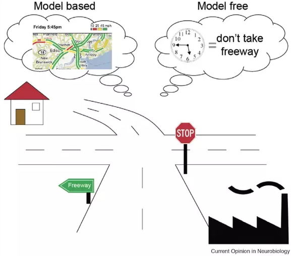
In the model-free (MF) RL methods seen sofar, we did not need to know anything about the dynamics of the environment to start learning a policy:
p(s' | s, a) \; \; r(s, a, s')
We just sampled transitions (s, a, r, s') and update the value / policy network. The main advantage is that the agent does not need to “think” when acting: it just select the action with highest Q-value or the one selected by the policy network (reflexive behavior). The other advantage is that you can use MF methods on any MDP: you do not need to know anything about them before applying MF as a blackbox optimizer.
However, MF methods are very slow (sample complexity): as they make no assumption, they have to learn everything by trial-and-error from scratch. If you had a model of the environment, you could plan ahead (what would happen if I did that?) and speed up learning (do not explore obviously stupid ideas): such a behavior is called model-based RL (MB). Dynamic programming (Section Dynamic programming) is for example a model-based method, as it requires the knowledge of p(s' | s, a) and r(s, a, s') to solve the Bellman equations.
In chess, for example, players plan ahead the possible moves up to a certain horizon and evaluate moves based on their emulated consequences. In real-time strategy games, learning the environment (world model) is part of the strategy: you do not attack right away.
This chapter presents several MB algorithms, including MPC planning algorithms, World models and the different variants of AlphaGo. We first present the main distinction in MB RL, planning algorithms (MPC) versus MB-augmented MF (Dyna) methods. Another useful dichotomy that we will see in the AlphaGo section is about learned models vs. given models.
Learning a dynamics model
Learning the world model is not complicated in theory. We just need to collect enough transitions (s, a, r , s') using a random agent (or an expert) and train a supervised model to predict the next state and the corresponding reward.
M(s, a) = (s', r )
Such a model is called the dynamics model, the transition model or the forward model, and basically answers the question:
What would happen if I did that?
The model can be deterministic (in which case we should use neural networks) or stochastic (in which case we should use Gaussian processes, mixture density networks or recurrent state space models). Any kind of supervised learning method can be used in principle.
Once you have trained a good transition model, you can generate rollouts, i.e. imaginary trajectories / episodes \tau using the model. Given an initial state s_0 and a policy \pi, you can unroll the future using the model s', r = M(s, a).
s_0 \xrightarrow[\pi]{} a_0 \xrightarrow[M]{} s_1 \xrightarrow[\pi]{} a_1 \xrightarrow[\pi]{} s_2 \xrightarrow[]{} \ldots \xrightarrow[M]{} s_T
Given the model, you can also compute the return R(\tau) of the emulated trajectory. Everything is as if you were interacting with the environment, but you actually do not need it anymore: the model becomes the environment. You can now search for an optimal policy on these emulated trajectories:
Any method can be used to optimize the policy. We can obviously use a model-free algorithm to maximize the expected return of the trajectories:
\mathcal{J}(\pi) = \mathbb{E}_{\tau \sim \rho_\pi}[R(\tau)]
The only sample complexity is the one needed to train the model: the rest is emulated. For problems where a physical step (t \rightarrow t+1) is very expensive compared to an inference step of the model (neural networks can predict very fast), this can even allow to use inefficient but optimal methods to find the policy. Brute-force optimization becomes possible if using the model is much faster that the real environment. However, this approach has two major drawbacks:
- The model can only be as good as the data, and errors are going to accumulate, especially for long trajectories or probabilistic MDPs.
- If the dataset does not contain the important transitions (for example where there are sparse rewards), the policy will likely be sub-optimal. In extreme cases, training the model up to a sufficient precision might necessitate more samples than learning the policy directly with MF methods.

