Deep Q-network (DQN)

Limitations of deep neural networks for function approximation

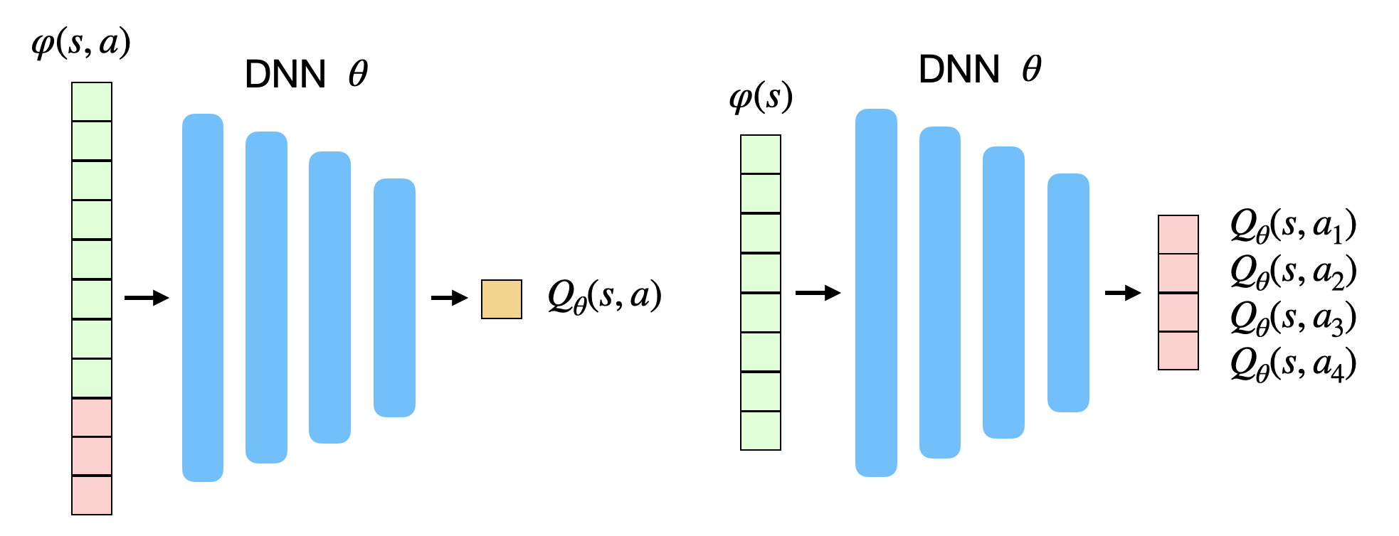
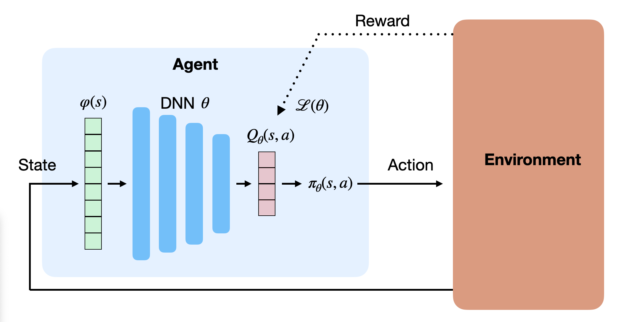
The goal of value-based deep RL is to approximate the Q-value of each possible state-action pair using a deep neural network. As shown on Figure 8.1, the network can either take a state-action pair as input and return a single output value, or take only the state as input and return the Q-value of all possible actions (only possible if the action space is discrete). In both cases, the goal is to learn estimates Q_\theta(s, a) with a NN with parameters \theta.

Figure 8.1: Function approximators can either associate a state-action pair (s, a) to its Q-value (left), or associate a state s to the Q-values of all actions possible in that state (right).

When using Q-learning, we have already seen that the problem is a regression problem, where the following mse loss function has to be minimized:

\mathcal{L}(\theta) = \mathbb{E}_{(s, a, r ,s')}[(r(s, a, s') + \gamma \, \max_{a'} Q_\theta(s', a') - Q_\theta(s, a))^2]

In short, we want to reduce the prediction error, i.e. the mismatch between the estimate of the value of an action Q_\theta(s, a) and the real return Q^\pi(s, a), here approximated with r(s, a, s') + \gamma \, \text{max}_{a'} Q_\theta(s', a').

Figure 8.2: Value-based Q-learning agent.

We can compute this loss by gathering enough samples (s, a, r, s') (i.e. single transitions), concatenating them randomly in minibatches, and let the DNN learn to minimize the prediction error using backpropagation and SGD, indirectly improving the policy. The following pseudocode would describe the training procedure when gathering transitions online, i.e. when directly interacting with the environment:

Naive Q-learning with function approximation

• Initialize value network Q_{\theta} with random weights.

• Initialize empty minibatch \mathcal{D} of maximal size n.

• Observe the initial state s_0.

• for t \in [0, T_\text{total}]:

  • Select the action a_t based on the behavior policy derived from Q_\theta(s_t, a) (e.g. softmax).

  • Perform the action a_t and observe the next state s_{t+1} and the reward r_{t+1}.

  • Store (s_t, a_t, r_{t+1}, s_{t+1}) in the minibatch.

  • When minibatch \mathcal{D} is full:

    • Train the value network Q_{\theta} on \mathcal{D} to minimize

    \mathcal{L}(\theta) = \mathbb{E}_\mathcal{D}[(r(s, a, s') + \gamma \, \text{max}_{a'} Q_\theta(s', a') - Q_\theta(s, a))^2]

    • Empty the minibatch \mathcal{D}.

However, the definition of the loss function uses the mathematical expectation operator E over all transitions, which can only be approximated by randomly sampling the distribution (the MDP). This implies that the samples concatenated in a minibatch should be independent from each other (i.i.d).

Correlated inputs

When gathering transitions online, the samples are correlated: (s_t, a_t, r_{t+1}, s_{t+1}) will be followed by (s_{t+1}, a_{t+1}, r_{t+2}, s_{t+2}), etc. When playing video games, two successive frames will be very similar (a few pixels will change, or even none if the sampling rate is too high) and the optimal action will likely not change either (to catch the ball in pong, you will need to perform the same action - going left - many times in a row).

Figure 8.3: Sucessive frames in a video game are highly correlated.

Correlated inputs/outputs are very bad for deep neural networks: the DNN will overfit and fall into a very bad local minimum. That is why stochastic gradient descent works so well: it randomly samples values from the training set to form minibatches and minimize the loss function on these uncorrelated samples (hopefully). If all samples of a minibatch were of the same class (e.g. zeros in MNIST), the network would converge poorly. This is the first problem preventing an easy use of deep neural networks as function approximators in RL.

Non-stationary targets

The second major problem is the non-stationarity of the targets in the loss function. In classification or regression, the desired values \mathbf{t} are fixed throughout learning: the class of an object does not change in the middle of the training phase.

\mathcal{L}(\theta) = - \mathbb{E}_{\mathbf{x}, \mathbf{t} \in \mathcal{D}}[ ||\mathbf{t} - \mathbf{y}||^2]

In Q-learning, the target :

t = r(s, a, s') + \gamma \, \max_{a'} Q_\theta(s', a')

will change during learning, as Q_\theta(s', a') depends on the weights \theta and will hopefully increase as the performance improves. This is the second problem of deep RL: deep NN are particularly bad on non-stationary problems, especially feedforward networks. They iteratively converge towards the desired value, but have troubles when the target also moves (like a dog chasing its tail).

Figure 8.4: In supervised learning, the targets are stationary, leading to good convergence properties. In RL, the targets are non-stationary and depending on the network itself. This often leads to suboptimal convergence.

Deep Q-Network (DQN)

Mnih et al. (2015) (originally arXived in Mnih et al. (2013)) proposed an elegant solution to the problems of correlated inputs/outputs and non-stationarity inherent to RL. This article is a milestone of deep RL and it is fair to say that it started the hype for deep RL.

Experience replay memory

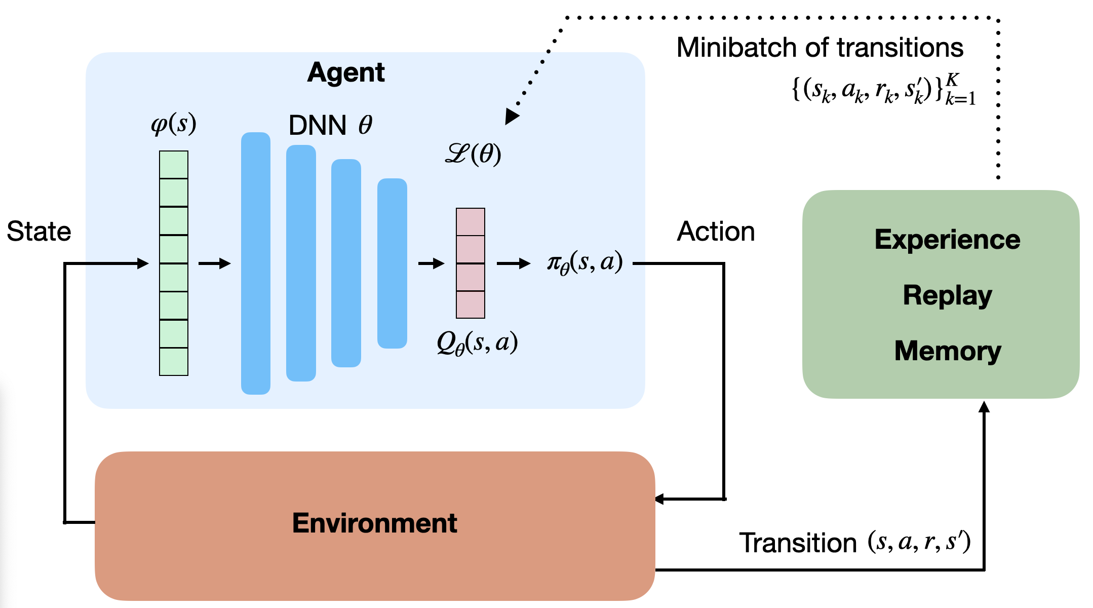
The first idea proposed by Mnih et al. (2015) solves the problem of correlated input/outputs and is actually quite simple: instead of feeding successive transitions into a minibatch and immediately training the NN on it, transitions are stored in a huge buffer called experience replay memory (ERM) or replay buffer able to store 100000 transitions. When the buffer is full, new transitions replace the old ones. SGD can now randomly sample the ERM to form minibatches and train the NN.

Figure 8.5: Experience replay memory. Interactions with the environment are stored in the ERM. Random minibatches are sampled from it to train the DQN value network.

The loss minimized by DQN is defined on a minibatch of size K:

\mathcal{L}(\theta) = \dfrac{1}{K} \, \sum_{k=1}^K (r_k + \gamma \, \text{max}_{a'} Q_\theta(s'_k, a') - Q_\theta(s_k, a_k))^2

Are these K samples i.i.d? They are independent because they are randomly sampled from the ERM, but they do not come from the same distribution: some were generated by a very old policy, some much more recently… However, this does not matter, as Q-learning is off-policy: the different policies that populated the ERM are a behavior policy, different from the learned one. Off-policy methods do not mind if the samples come from the same distribution or not. It would be very different if we has used SARSA instead.

→ It is only possible to use an experience replay memory with off-policy algorithms

Target networks

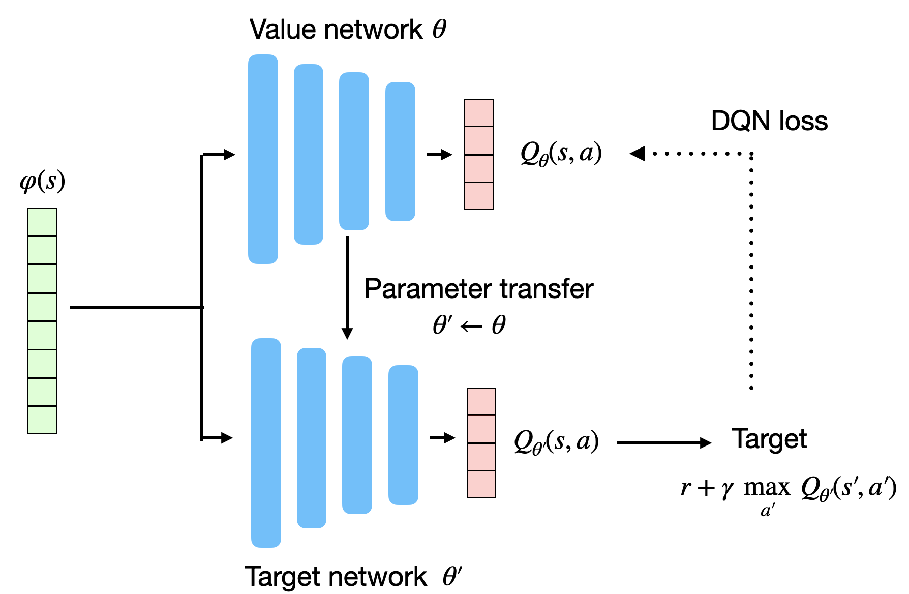
The second idea solves the non-stationarity of the targets r(s, a, s') + \gamma \, \max_{a'} Q_\theta(s', a'). Instead of computing it with the current parameters \theta of the NN, they are computed with an old version of the NN called the target network with parameters \theta'.

\mathcal{L}(\theta) = \dfrac{1}{K} \, \sum_{k=1}^K (r_k + \gamma \, \text{max}_{a'} Q_{\theta'}(s'_k, a') - Q_\theta(s_k, a_k))^2

The target network is updated only infrequently (every thousands of iterations or so) with the learned weights \theta. As this target network does not change very often, the targets stay constant for a long period of time, and the problem becomes more stationary.

Figure 8.6: The target network is used to compute the targets to train the value network. Its waits are regularly copied from the value network.

Figure 8.7: By keeping the the targets constant for a while, the target network lets the value network catch up with them and converge optimally (in principle).

DQN algorithm

The resulting algorithm is called Deep Q-Network (DQN). It is summarized by the following pseudocode:

DQN algorithm

• Initialize value network Q_{\theta} with random weights.

• Copy Q_{\theta} to create the target network Q_{\theta'}.

• Initialize experience replay memory \mathcal{D} of maximal size N.

• Observe the initial state s_0.

• for t \in [0, T_\text{total}]:

  • Select the action a_t based on the behavior policy derived from Q_\theta(s_t, a) (e.g. softmax).

  • Perform the action a_t and observe the next state s_{t+1} and the reward r_{t+1}.

  • Store (s_t, a_t, r_{t+1}, s_{t+1}) in the experience replay memory.

  • Every T_\text{train} steps:

    • Sample a minibatch \mathcal{D}_s randomly from \mathcal{D}.

    • For each transition (s, a, r, s') in the minibatch:

      • Predict the Q-value of the greedy action in the next state \max_{a'} Q_{\theta'}(s', a') using the target network.

      • Compute the target value t = r + \gamma \, \max_{a'} Q_{\theta'}(s', a').

    • Train the value network Q_{\theta} on \mathcal{D}_s to minimize \mathcal{L}(\theta) = \mathbb{E}_{\mathcal{D}_s}[(t - Q_\theta(s, a))^2]

  • Every T_\text{target} steps:

    • Update the target network with the trained value network: \theta' \leftarrow \theta

The first thing to notice is that experienced transitions are not immediately used for learning, but simply stored in the ERM to be sampled later. Due to the huge size of the ERM, it is even likely that the recently experienced transition will only be used for learning hundreds or thousands of steps later. Meanwhile, very old transitions, generated using an initially bad policy, can be used to train the network for a very long time.

The second thing is that the target network is not updated very often (T_\text{target}=10000), so the target values are going to be wrong a long time. More recent algorithms such as DDPG use a smoothed version of the current weights, as proposed in Lillicrap et al. (2015):

\theta' = \tau \, \theta + (1-\tau) \, \theta'

If this rule is applied after each step with a very small rate \tau, the target network will slowly track the learned network, but never be the same. Modern implementations of DQN use this smoothed version.

These two facts make DQN extremely slow to learn: millions of transitions are needed to obtain a satisfying policy. This is called the sample complexity, i.e. the number of transitions needed to obtain a satisfying performance. DQN finds very good policies, but at the cost of a very long training time.

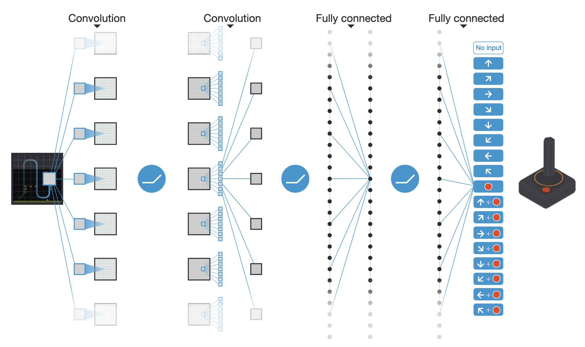
DQN was initially applied to solve various Atari 2600 games. Video frames were used as observations and the set of possible discrete actions was limited (left/right/up/down, shoot, etc). The CNN used is depicted on Figure 8.8. It has two convolutional layers, no max-pooling, 2 fully-connected layer and one output layer representing the Q-value of all possible actions in the games.

Figure 8.8: Architecture of the CNN used in the original DQN paper. Source: Mnih et al. (2015).

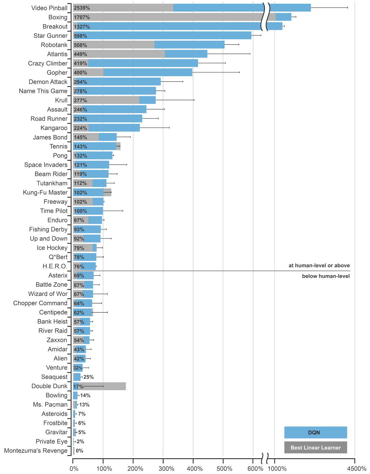
The problem of partial observability (a single frame does not hold the Markov property) is solved by concatenating the four last video frames into a single tensor used as input to the CNN. The convolutional layers become able through learning to extract the speed information from it. Some of the Atari games (Pinball, Breakout) were solved with a performance well above human level, especially when they are mostly reactive. Games necessitating more long-term planning (Montezuma’s Revenge) were still poorly learned, though.

Why no max-pooling?

The CNN used in deep RL agents (DQN or others) usually do not have many max-pooling layers (or strides, which are equivalent). The goal of a max-pooling layer is to achieve spatial invariance, i.e. being able to recognize an object whatever its position in the input image. A cat is a cat, whether it is on the left or the right of the image.

However, we usually do not want spatial invariance in RL: the location of the ball in the frame in Breakout or Pinball is extremely important for the policy, we do not want to get rid of it.

The drawback of not having max-pooling layers is that the last convolutional layer (before the first FC layer) will still have a lot of elements, so the first FC matrix will likely be huge. This limits the ability of deep RL algorithms to work with big images.

Beside being able to learn using delayed and sparse rewards in highly dimensional input spaces, the true tour de force of DQN is that it was able to learn the 49 Atari games using the same architecture and hyperparameters, showing the generality of the approach.

Figure 8.9: Results on the Atari benchmark. Some games achieved super-human performance. Source: Mnih et al. (2015)

Lillicrap, T. P., Hunt, J. J., Pritzel, A., Heess, N., Erez, T., Tassa, Y., et al. (2015). Continuous control with deep reinforcement learning. CoRR. Available at: http://arxiv.org/abs/1509.02971.

Mnih, V., Kavukcuoglu, K., Silver, D., Graves, A., Antonoglou, I., Wierstra, D., et al. (2013). Playing Atari with Deep Reinforcement Learning. Available at: http://arxiv.org/abs/1312.5602.

Mnih, V., Kavukcuoglu, K., Silver, D., Rusu, A. A., Veness, J., Bellemare, M. G., et al. (2015). Human-level control through deep reinforcement learning. Nature 518, 529–533. doi:10.1038/nature14236.