.md .pdf

Contents

2. Linear Regression

Slides: pdf

2.1. Linear regression

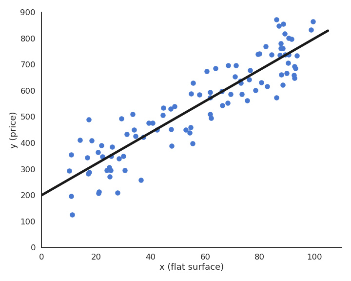
Fig. 2.23 Simple linear regression. \(x\) is the input, \(y\) the output. The data is represented by blue dots, the model by the black line.

Let’s consider a training set of N examples \(\mathcal{D} = (x_i, t_i)_{i=1..N}\). In linear regression, we want to learn a linear model (hypothesis) \(y\) that is linearly dependent on the input \(x\):

\[ y = f_{w, b}(x) = w \, x + b \]

The free parameters of the model are the slope \(w\) and the intercept \(b\). This model corresponds to a single artificial neuron with output \(y\), having one input \(x\), one weight \(w\), one bias \(b\) and a linear activation function \(f(x) = x\).

Fig. 2.24 Artificial neuron with multiple inputs.

The goal of the linear regression (or least mean squares - LMS) is to minimize the mean square error (mse) between the targets and the predictions. This loss function is defined as the mathematical expectation of the quadratic error over the training set:

\[ \mathcal{L}(w, b) = \mathbb{E}_{x_i, t_i \in \mathcal{D}} [ (t_i - y_i )^2 ] \]

As the training set is finite and the samples i.i.d, we can simply replace the expectation by an average over the training set:

\[ \mathcal{L}(w, b) = \frac{1}{N} \, \sum_{i=1}^{N} (t_i - y_i )^2 \]

The minimum of the mse is achieved when the prediction \(y_i = f_{w, b}(x_i)\) is equal to the true value \(t_i\) for all training examples. In other words, we want to minimize the residual error of the model on the data. It is not always possible to obtain the global minimum (0) as the data may be noisy, but the closer, the better.

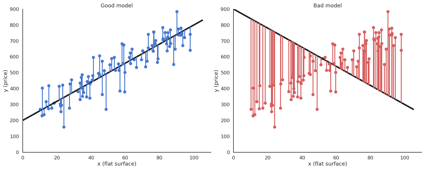
Fig. 2.25 A good fit to the data is when the prediction \(y_i\) (on the line) is close to the data \(t_i\) for all training examples.

2.1.1. Least Mean Squares

We search for \(w\) and \(b\) which minimize the mean square error:

\[ \mathcal{L}(w, b) = \frac{1}{N} \, \sum_{i=1}^{N} (t_i - y_i )^2 \]

We will apply gradient descent to iteratively modify estimates of \(w\) and \(b\):

\[ \Delta w = - \eta \, \frac{\partial \mathcal{L}(w, b)}{\partial w} \]

\[ \Delta b = - \eta \, \frac{\partial \mathcal{L}(w, b)}{\partial b} \]

Let’s search for the partial derivative of the mean square error with respect to \(w\):

\[ \frac{\partial \mathcal{L}(w, b)}{\partial w} = \frac{\partial}{\partial w} [\frac{1}{N} \, \sum_{i=1}^{N} (t_i - y_i )^2] \]

Partial derivatives are linear, so the derivative of a sum is the sum of the derivatives:

\[ \frac{\partial \mathcal{L}(w, b)}{\partial w} = \frac{1}{N} \, \sum_{i=1}^{N} \frac{\partial}{\partial w} (t_i - y_i )^2 \]

This means we can compute a gradient for each training example instead of for the whole training set (see later the distinction batch/online):

\[ \frac{\partial \mathcal{L}(w, b)}{\partial w} = \frac{1}{N} \, \sum_{i=1}^{N} \frac{\partial}{\partial w} \mathcal{l}_i(w, b) \qquad \text{with} \qquad \mathcal{l}_i(w, b) = (t_i - y_i )^2 \]

The individual loss \(\mathcal{l}_i(w, b) = (t_i - y_i )^2\) is the composition of two functions:

• a square error function \(g_i(y_i) = (t_i - y_i)^2\).

• the prediction \(y_i = f_{w, b}(x_i) = w \, x_i + b\).

The chain rule tells us how to derive such composite functions:

\[ \frac{ d f(g(x))}{dx} = \frac{ d f(g(x))}{d g(x)} \times \frac{ d g(x)}{dx} = \frac{ d f(y)}{dy} \times \frac{ d g(x)}{dx} \]

The first derivative considers \(g(x)\) to be a single variable. Applied to our problem, this gives:

\[ \frac{\partial}{\partial w} \mathcal{l}_i(w, b) = \frac{\partial g_i(y_i)}{\partial y_i} \times \frac{\partial y_i}{\partial w} \]

The square error function \(g_i(y) = (t_i - y)^2\) is easy to differentiate w.r.t \(y\):

\[ \frac{\partial g_i(y_i)}{\partial y_i} = - 2 \, (t_i - y_i) \]

The prediction \(y_i = w \, x_i + b\) also w.r.t \(w\) and \(b\):

\[ \frac{\partial y_i}{\partial w} = x_i \]

\[ \frac{\partial y_i}{\partial b} = 1 \]

The partial derivative of the individual loss is:

\[ \frac{\partial \mathcal{l}_i(w, b)}{\partial w} = - 2 \, (t_i - y_i) \, x_i \]

\[ \frac{\partial \mathcal{l}_i(w, b)}{\partial b} = - 2 \, (t_i - y_i) \]

This gives us:

\[ \frac{\partial \mathcal{L}(w, b)}{\partial w} = - \frac{2}{N} \sum_{i=1}^{N} (t_i - y_i) \, x_i \]

\[ \frac{\partial \mathcal{L}(w, b)}{\partial b} = - \frac{2}{N} \sum_{i=1}^{N} (t_i - y_i) \]

Gradient descent is then defined by the learning rules (absorbing the 2 in \(\eta\)):

\[ \Delta w = \eta \, \frac{1}{N} \sum_{i=1}^{N} (t_i - y_i) \, x_i \]

\[ \Delta b = \eta \, \frac{1}{N} \sum_{i=1}^{N} (t_i - y_i) \]

Least Mean Squares (LMS) or Ordinary Least Squares (OLS) is a batch algorithm: the parameter changes are computed over the whole dataset.

\[ \Delta w = \eta \, \frac{1}{N} \sum_{i=1}^{N} (t_i - y_i) \, x_i \]

\[ \Delta b = \eta \, \frac{1}{N} \sum_{i=1}^{N} (t_i - y_i) \]

The parameter changes have to be applied multiple times (epochs) in order for the parameters to converge. One can stop when the parameters do not change much, or after a fixed number of epochs.

LMS algorithm

• \(w=0 \quad;\quad b=0\)

• for M epochs:

  • \(dw=0 \quad;\quad db=0\)

  • for each sample \((x_i, t_i)\):

    • \(y_i = w \, x_i + b\)

    • \(dw = dw + (t_i - y_i) \, x_i\)

    • \(db = db + (t_i - y_i)\)

  • \(\Delta w = \eta \, \frac{1}{N} dw\)

  • \(\Delta b = \eta \, \frac{1}{N} db\)

Fig. 2.26 Visualization of least mean squares applied to a simple regression problem with \(\eta=0.1\). Each step of the animation corresponds to one epoch (iteration over the training set).

During learning, the mean square error (mse) decreases with the number of epochs but does not reach zero because of the noise in the data.

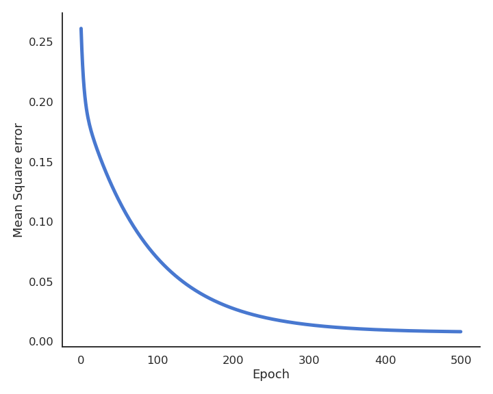
Fig. 2.27 Evolution of the loss function during training.

2.1.2. Delta learning rule

LMS is very slow, because it changes the weights only after the whole training set has been evaluated. It is also possible to update the weights immediately after each example using the delta learning rule, which is the online version of LMS:

\[\Delta w = \eta \, (t_i - y_i) \, x_i\]

\[\Delta b = \eta \, (t_i - y_i)\]

Delta learning rule

• \(w=0 \quad;\quad b=0\)

• for M epochs:

  • for each sample \((x_i, t_i)\):

    • \(y_i = w \, x_i + b\)

    • \(\Delta w = \eta \, (t_i - y_i ) \, x_i\)

    • \(\Delta b = \eta \, (t_i - y_i)\)

The batch version is more stable, but the online version is faster: the weights have already learned something when arriving at the end of the first epoch. Note that the loss function is slightly higher at the end of learning (see Exercise 3 for a deeper discussion).

Fig. 2.28 Visualization of the delta learning rule applied to a simple regression problem with \(\eta = 0.1\). Each step of the animation corresponds to one epoch (iteration over the training set).

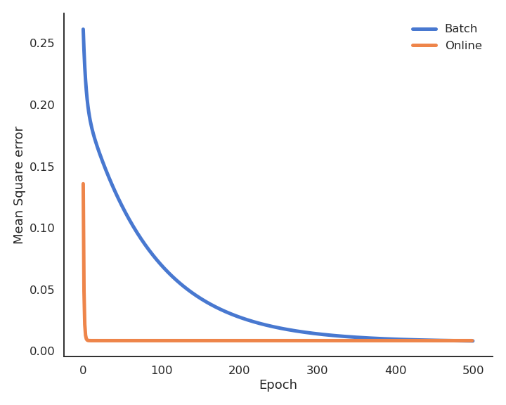
Fig. 2.29 Evolution of the loss function during training. With the same learning rate, the delta learning rule converges much faster but reaches a poorer minimum. Lowering the learning rate slows down learning but reaches a better minimum.

2.2. Multiple linear regression

The key idea of linear regression (one input \(x\), one output \(y\)) can be generalized to multiple inputs and outputs.

Multiple Linear Regression (MLR) predicts several output variables based on several explanatory variables:

\[\begin{split} \begin{cases} y_1 = w_1 \, x_1 + w_2 \, x_2 + b_1\\ \\ y_2 = w_3 \, x_1 + w_3 \, x_2 + b_2\\ \end{cases} \end{split}\]

Example: fuel consumption and CO2 emissions

Let’s suppose you have 13971 measurements in some Excel file, linking engine size, number of cylinders, fuel consumption and CO2 emissions of various cars. You want to predict fuel consumption and CO2 emissions when you know the engine size and the number of cylinders.

Engine size	Cylinders	Fuel consumption	CO2 emissions
2	4	8.5	196
2.4	4	9.6	221
1.5	4	5.9	136
3.5	6	11	255
…	…	…	…

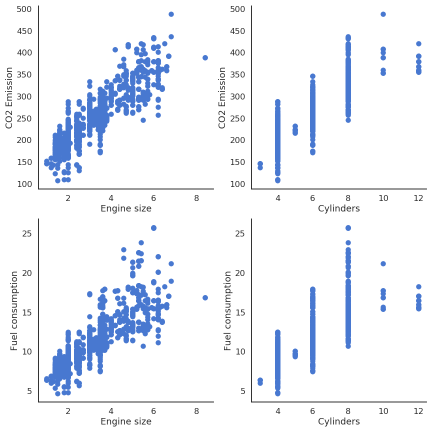
Fig. 2.30 CO2 emissions and fuel consumption depend almost linearly on the engine size and number of cylinders.

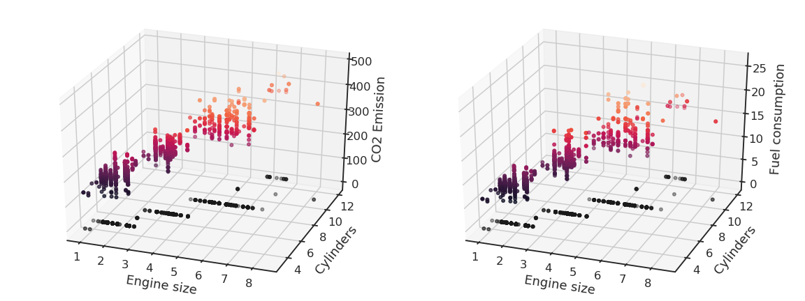
Fig. 2.31 CO2 emissions and fuel consumption depend almost linearly on the engine size and number of cylinders.

We can notice that the output variables seem to linearly depend on the inputs. Noting the input variables \(x_1\), \(x_2\) and the output ones \(y_1\), \(y_2\), we can define our problem as a multiple linear regression:

\[\begin{split} \begin{cases} y_1 = w_1 \, x_1 + w_2 \, x_2 + b_1\\ \\ y_2 = w_3 \, x_1 + w_3 \, x_2 + b_2\\ \end{cases} \end{split}\]

and solve it using the least mean squares method by minimizing the mse between the model and the data.

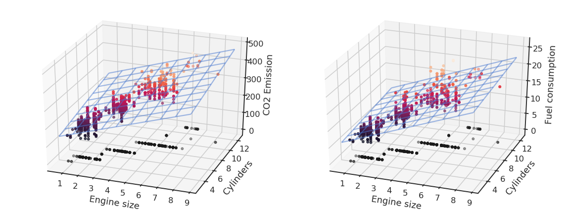
Fig. 2.32 The result of MLR is a plane in the input space.

Note

Using the Python library scikit-learn (https://scikit-learn.org), this is done in two lines of code:

from sklearn.linear_model import LinearRegression
reg = LinearRegression().fit(X, y)

The system of equations:

\[\begin{split} \begin{cases} y_1 = w_1 \, x_1 + w_2 \, x_2 + b_1\\ \\ y_2 = w_3 \, x_1 + w_4 \, x_2 + b_2\\ \end{cases} \end{split}\]

can be put in a matrix-vector form:

\[\begin{split} \begin{bmatrix} y_1 \\ y_2 \\\end{bmatrix} = \begin{bmatrix} w_1 & w_2 \\ w_3 & w_4 \\\end{bmatrix} \times \begin{bmatrix} x_1 \\ x_2 \\\end{bmatrix} + \begin{bmatrix} b_1 \\ b_2 \\\end{bmatrix} \end{split}\]

We simply create the corresponding vectors and matrices:

\[\begin{split} \mathbf{x} = \begin{bmatrix} x_1 \\ x_2 \\\end{bmatrix} \qquad \mathbf{y} = \begin{bmatrix} y_1 \\ y_2 \\\end{bmatrix} \qquad \mathbf{t} = \begin{bmatrix} t_1 \\ t_2 \\\end{bmatrix} \qquad \mathbf{b} = \begin{bmatrix} b_1 \\ b_2 \\\end{bmatrix} \qquad W = \begin{bmatrix} w_1 & w_2 \\ w_3 & w_4 \\\end{bmatrix} \end{split}\]

\(\mathbf{x}\) is the input vector, \(\mathbf{y}\) is the output vector, \(\mathbf{t}\) is the target vector. \(W\) is called the weight matrix and \(\mathbf{b}\) the bias vector.

The model is now defined by:

\[ \mathbf{y} = f_{W, \mathbf{b}}(\mathbf{x}) = W \times \mathbf{x} + \mathbf{b} \]

The problem is exactly the same as before, except that we use vectors and matrices instead of scalars: \(\mathbf{x}\) and \(\mathbf{y}\) can have any number of dimensions, the same procedure will apply. This corresponds to a linear neural network (or linear perceptron), with one output neuron per predicted value \(y_i\) using the linear activation function.

Fig. 2.33 A linear perceptron is a single layer of artificial neurons. The output vector \(\mathbf{y}\) is compared to the ground truth vector \(\mathbf{t}\) using the mse loss.

The mean square error still needs to be a scalar in order to be minimized. We can define it as the squared norm of the error vector:

\[ \min_{W, \mathbf{b}} \, \mathcal{L}(W, \mathbf{b}) = \mathbb{E}_\mathcal{D} [ ||\mathbf{t} - \mathbf{y}||^2 ] = \mathbb{E}_\mathcal{D} [ ((t_1 - y_1)^2 + (t_2 - y_2)^2) ] \]

In order to apply gradient descent, one needs to calculate partial derivatives w.r.t the weight matrix \(W\) and the bias vector \(\mathbf{b}\), i.e. gradients:

\[\begin{split} \begin{cases} \Delta W = - \eta \, \nabla_W \, \mathcal{L}(W, \mathbf{b}) \\ \\ \Delta \mathbf{b} = - \eta \, \nabla_\mathbf{b} \mathcal{L}(W, \mathbf{b}) \\ \end{cases} \end{split}\]

Note

Some more advanced linear algebra becomes important to know how to compute these gradients:

https://web.stanford.edu/class/cs224n/readings/gradient-notes.pdf

We search the minimum of the mse loss function:

\[ \min_{W, \mathbf{b}} \, \mathcal{L}(W, \mathbf{b}) = \mathbb{E}_\mathcal{D} [ ||\mathbf{t} - \mathbf{y}||^2 ] \approx \frac{1}{N} \, \sum_{i=1}^N ||\mathbf{t}_i - \mathbf{y}_i||^2 = \frac{1}{N} \, \sum_{i=1}^N \mathcal{l}_i(W, \mathbf{b}) \]

The individual loss function \(\mathcal{l}_i(W, \mathbf{b})\) is the squared \(\mathcal{L}^2\)-norm of the error vector, what can be expressed as a dot product or a vector multiplication:

\[ \mathcal{l}_i(W, \mathbf{b}) = ||\mathbf{t}_i - \mathbf{y}_i||^2 = \langle \mathbf{t}_i - \mathbf{y}_i \cdot \mathbf{t}_i - \mathbf{y}_i \rangle = (\mathbf{t}_i - \mathbf{y}_i)^T \times (\mathbf{t}_i - \mathbf{y}_i) \]

Note

Remember:

\[\begin{split}\mathbf{x}^T \times \mathbf{x} = \begin{bmatrix} x_1 & x_2 & \ldots & x_n \end{bmatrix} \times \begin{bmatrix} x_1 \\ x_2 \\ \vdots \\ x_n \end{bmatrix} = x_1 \, x_1 + x_2 \, x_2 + \ldots + x_n \, x_n = \langle \mathbf{x} \cdot \mathbf{x} \rangle = ||\mathbf{x}||^2_2\end{split}\]

The chain rule tells us in principle that:

\[\nabla_{W} \, \mathcal{l}_i(W, \mathbf{b}) = \nabla_{\mathbf{y}_i} \, \mathcal{l}_i(W, \mathbf{b}) \times \nabla_{W} \, \mathbf{y}_i\]

The gradient w.r.t the output vector \(\mathbf{y}_i\) is quite easy to obtain, as it a quadratic function of \(\mathbf{t}_i - \mathbf{y}_i\):

\[\nabla_{\mathbf{y}_i} \, \mathcal{l}_i(W, \mathbf{b}) = \nabla_{\mathbf{y}_i} \, (\mathbf{t}_i - \mathbf{y}_i)^T \times (\mathbf{t}_i - \mathbf{y}_i)\]

The proof relies on product differentiation \((f\times g)' = f' \, g + f \, g'\):

\[\begin{split}\begin{aligned} \nabla_{\mathbf{y}_i} \, (\mathbf{t}_i - \mathbf{y}_i)^T \times (\mathbf{t}_i - \mathbf{y}_i) & = ( \nabla_{\mathbf{y}_i} \, (\mathbf{t}_i - \mathbf{y}_i) ) \times (\mathbf{t}_i - \mathbf{y}_i) + (\mathbf{t}_i - \mathbf{y}_i) \times \nabla_{\mathbf{y}_i} \, (\mathbf{t}_i - \mathbf{y}_i) \\ &\\ &= - (\mathbf{t}_i - \mathbf{y}_i) - (\mathbf{t}_i - \mathbf{y}_i) \\ &\\ &= - 2 \, (\mathbf{t}_i - \mathbf{y}_i) \\ \end{aligned} \end{split}\]

Note

We use the properties \(\nabla_{\mathbf{x}}\, \mathbf{x}^T \times \mathbf{z} = \mathbf{z}\) and \(\nabla_{\mathbf{z}} \, \mathbf{x}^T \times \mathbf{z} = \mathbf{x}\) to get rid of the transpose.

The “problem” is when computing \(\nabla_{W} \, \mathbf{y}_i = \nabla_{W} \, (W \times \mathbf{x}_i + \mathbf{b})\):

• \(\mathbf{y}_i\) is a vector and \(W\) a matrix.

• \(\nabla_{W} \, \mathbf{y}_i\) is then a Jacobian (matrix), not a gradient (vector).

Intuitively, differentiating \(W \times \mathbf{x}_i + \mathbf{b}\) w.r.t \(W\) should return \(\mathbf{x}_i\), but it is a vector, not a matrix…

Actually, only the gradient (or Jacobian) of \(\mathcal{l}_i(W, \mathbf{b})\) w.r.t \(W\) should be a matrix of the same size as \(W\) so that we can apply gradient descent:

\[\Delta W = - \eta \, \nabla_W \, \mathcal{L}(W, \mathbf{b})\]

We already know that:

\[\nabla_{W} \, \mathcal{l}_i(W, \mathbf{b}) = - 2\, (\mathbf{t}_i - \mathbf{y}_i) \times \nabla_{W} \, \mathbf{y}_i\]

If \(\mathbf{x}_i\) has \(n\) elements and \(\mathbf{y}_i\) \(m\) elements, \(W\) is a \(m \times n\) matrix.

Note

Remember the outer product between two vectors:

\[\begin{split} \mathbf{u} \times \mathbf{v}^\textsf{T} = \begin{bmatrix}u_1 \\ u_2 \\ u_3 \\ u_4\end{bmatrix} \begin{bmatrix}v_1 & v_2 & v_3\end{bmatrix} = \begin{bmatrix} u_1v_1 & u_1v_2 & u_1v_3 \\ u_2v_1 & u_2v_2 & u_2v_3 \\ u_3v_1 & u_3v_2 & u_3v_3 \\ u_4v_1 & u_4v_2 & u_4v_3 \end{bmatrix}. \end{split}\]

It is easy to see that the outer product between \((\mathbf{t}_i - \mathbf{y}_i)\) and \(\mathbf{x}_i\) gives a \(m \times n\) matrix:

\[\begin{split} \nabla_W \, \mathcal{l}_i(W, \mathbf{b}) = - 2 \, (\mathbf{t}_i - \mathbf{y}_i) \times \mathbf{x}_i^T\\ \end{split}\]

Let’s prove it element per element on a small matrix:

\[ \mathbf{y} = W \times \mathbf{x} + \mathbf{b} \]

\[\begin{split} \begin{bmatrix} y_1 \\ y_2 \\\end{bmatrix} = \begin{bmatrix} w_1 & w_2 \\ w_3 & w_4 \\\end{bmatrix} \times \begin{bmatrix} x_1 \\ x_2 \\\end{bmatrix} + \begin{bmatrix} b_1 \\ b_2 \\\end{bmatrix} \end{split}\]

\[\begin{split} \mathcal{l}(W, \mathbf{b}) = (\mathbf{t} - \mathbf{y})^T \times (\mathbf{t} - \mathbf{y}) = \begin{bmatrix} t_1 - y_1 & t_2 - y_2 \\\end{bmatrix} \times \begin{bmatrix} t_1 - y_1 \\ t_2 - y_2 \\\end{bmatrix} = (t_1 - y_1)^2 + (t_2 - y_2)^2 \end{split}\]

The Jacobian w.r.t \(W\) can be explicitly formed using partial derivatives:

\[\begin{split} \nabla_W \, \mathcal{l}(W, \mathbf{b}) = \begin{bmatrix} \dfrac{\partial \mathcal{l}(W, \mathbf{b})}{\partial w_1} & \dfrac{\partial \mathcal{l}(W, \mathbf{b})}{\partial w_2} \\ \dfrac{\partial \mathcal{l}(W, \mathbf{b})}{\partial w_3} & \dfrac{\partial \mathcal{l}(W, \mathbf{b})}{\partial w_4} \\ \end{bmatrix} = \begin{bmatrix} -2 \, (t_1 - y_1) \, x_1 & -2 \, (t_1 - y_1) \, x_2 \\ -2 \, (t_2 - y_2) \, x_1 & -2 \, (t_2 - y_2) \, x_2 \\ \end{bmatrix} \end{split}\]

We can rearrange this matrix as an outer product:

\[\begin{split} \nabla_W \, \mathcal{l}(W, \mathbf{b}) = -2 \, \begin{bmatrix} t_1 - y_1 \\ t_2 - y_2 \\ \end{bmatrix} \times \begin{bmatrix} x_1 & x_2 \\ \end{bmatrix} = - 2 \, (\mathbf{t} - \mathbf{y}) \times \mathbf{x}^T \end{split}\]

Multiple linear regression

• Batch version:

\[\begin{split}\begin{cases} \Delta W = \eta \, \dfrac{1}{N} \sum_{i=1}^N \, (\mathbf{t}_i - \mathbf{y}_i ) \times \mathbf{x}_i^T \\ \\ \Delta \mathbf{b} = \eta \, \dfrac{1}{N} \sum_{i=1}^N \, (\mathbf{t}_i - \mathbf{y}_i) \\ \end{cases}\end{split}\]

• Online version (delta learning rule):

\[\begin{split}\begin{cases} \Delta W = \eta \, (\mathbf{t}_i - \mathbf{y}_i ) \times \mathbf{x}_i^T \\ \\ \Delta \mathbf{b} = \eta \, (\mathbf{t}_i - \mathbf{y}_i) \\ \end{cases}\end{split}\]

The matrix-vector notation is completely equivalent to having one learning rule per parameter:

\[\begin{split} \begin{cases} \Delta w_1 = \eta \, (t_1 - y_1) \, x_1 \\ \Delta w_2 = \eta \, (t_1 - y_1) \, x_2 \\ \Delta w_3 = \eta \, (t_2 - y_2) \, x_1 \\ \Delta w_4 = \eta \, (t_2 - y_2) \, x_2 \\ \end{cases} \qquad \begin{cases} \Delta b_1 = \eta \, (t_1 - y_1) \\ \Delta b_2 = \eta \, (t_2 - y_2) \\ \end{cases} \end{split}\]

Note

The delta learning rule is always of the form: \(\Delta w\) = eta * error * input. Biases have an input of 1.

2.3. Logistic regression

Let’s suppose we want to perform a regression, but where the outputs \(t_i\) are bounded between 0 and 1. We could use a logistic (or sigmoid) function instead of a linear function in order to transform the input into an output:

\[ y = \sigma(w \, x + b ) = \displaystyle\frac{1}{1+\exp(-w \, x - b )} \]

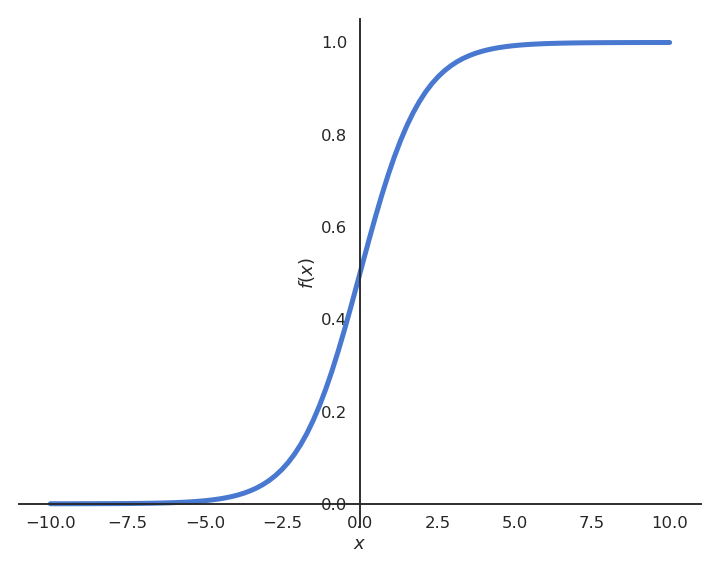
Fig. 2.34 Logistic or sigmoid function \(\sigma(x)=\displaystyle\frac{1}{1+\exp(-x)}\).

By definition of the logistic function, the prediction \(y\) will be bounded between 0 and 1, what matches the targets \(t\). Let’s now apply gradient descent on the mse loss using this new model. The individual loss will be:

\[l_i(w, b) = (t_i - \sigma(w \, x_i + b) )^2 \]

The partial derivative of the individual loss is easy to find using the chain rule:

\[\begin{split} \begin{aligned} \displaystyle\frac{\partial l_i(w, b)}{\partial w} &= 2 \, (t_i - y_i) \, \frac{\partial}{\partial w} (t_i - \sigma(w \, x_i + b ))\\ &\\ &= - 2 \, (t_i - y_i) \, \sigma'(w \, x_i + b ) \, x_i \\ \end{aligned} \end{split}\]

The non-linear transfer function \(\sigma(x)\) therefore adds its derivative into the gradient:

\[ \Delta w = \eta \, (t_i - y_i) \, \sigma'(w \, x_i + b ) \, x_i \]

The logistic function \(\sigma(x)=\frac{1}{1+\exp(-x)}\) has the nice property that its derivative can be expressed easily:

\[ \sigma'(x) = \sigma(x) \, (1 - \sigma(x) ) \]

Note

Here is the proof using the fact that the derivative of \(\displaystyle\frac{1}{f(x)}\) is \(\displaystyle\frac{- f'(x)}{f^2(x)}\) :

\[\begin{split}\begin{aligned} \sigma'(x) & = \displaystyle\frac{-1}{(1+\exp(-x))^2} \, (- \exp(-x)) \\ &\\ &= \frac{1}{1+\exp(-x)} \times \frac{\exp(-x)}{1+\exp(-x)}\\ &\\ &= \frac{1}{1+\exp(-x)} \times \frac{1 + \exp(-x) - 1}{1+\exp(-x)}\\ &\\ &= \frac{1}{1+\exp(-x)} \times (1 - \frac{1}{1+\exp(-x)})\\ &\\ &= \sigma(x) \, (1 - \sigma(x) )\\ \end{aligned} \end{split}\]

The delta learning rule for the logistic regression model is therefore easy to obtain:

\[\begin{split} \begin{cases} \Delta w = \eta \, (t_i - y_i) \, y_i \, ( 1 - y_i ) \, x_i \\ \\ \Delta b = \eta \, (t_i - y_i) \, y_i \, ( 1 - y_i ) \\ \end{cases} \end{split}\]

Generalized form of the delta learning rule

Fig. 2.35 Artificial neuron with multiple inputs.

For a linear perceptron with parameters \(W\) and \(\mathbf{b}\) and any activation function \(f\):

\[ \mathbf{y} = f(W \times \mathbf{x} + \mathbf{b} ) \]

and the mse loss function:

\[ \mathcal{L}(W, \mathbf{b}) = \mathbb{E}_{\mathcal{D}}[||\mathbf{t} - \mathbf{y}||^2] \]

the delta learning rule has the form:

\[\begin{split} \begin{cases} \Delta W = \eta \, (\mathbf{t} - \mathbf{y}) \times f'(W \times \mathbf{x} + \mathbf{b}) \times \mathbf{x}^T \\ \\ \Delta \mathbf{b} = \eta \, (\mathbf{t} - \mathbf{y}) \times f'(W \times \mathbf{x} + \mathbf{b}) \\ \end{cases} \end{split}\]

In the linear case, \(f'(x) = 1\). One can use any non-linear function, e.g hyperbolic tangent tanh(), ReLU, etc. Transfer functions are chosen for neural networks so that we can compute their derivative easily.

2.4. Polynomial regression

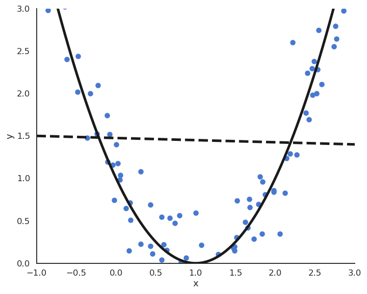
Fig. 2.36 Polynomial regression.

The functions underlying real data are rarely linear plus some noise around the ideal value. In the figure above, the input/output function is better modeled by a second-order polynomial:

\[y = f_{\mathbf{w}, b}(x) = w_1 \, x + w_2 \, x^2 +b\]

We can transform the input into a vector of coordinates:

\[\begin{split}\mathbf{x} = \begin{bmatrix} x \\ x^2 \\ \end{bmatrix} \qquad \mathbf{w} = \begin{bmatrix} w_1 \\ w_2 \\ \end{bmatrix}\end{split}\]

The problem becomes:

\[y = \langle \mathbf{w} . \mathbf{x} \rangle + b = \sum_j w_j \, x_j + b\]

We can simply apply multiple linear regression (MLR) to find \(\mathbf{w}\) and b:

\[\begin{split}\begin{cases} \Delta \mathbf{w} = \eta \, (t - y) \, \mathbf{x}\\ \\ \Delta b = \eta \, (t - y)\\ \end{cases}\end{split}\]

This generalizes to polynomials of any order \(p\):

\[y = f_{\mathbf{w}, b}(x) = w_1 \, x + w_2 \, x^2 + \ldots + w_p \, x^p + b\]

We create a vector of powers of \(x\):

\[\begin{split}\mathbf{x} = \begin{bmatrix} x \\ x^2 \\ \ldots \\ x^p \end{bmatrix} \qquad \mathbf{w} = \begin{bmatrix} w_1 \\ w_2 \\ \ldots \\ w_p \end{bmatrix}\end{split}\]

ad apply multiple linear regression (MLR) to find \(\mathbf{w}\) and b:

\[\begin{split}\begin{cases} \Delta \mathbf{w} = \eta \, (t - y) \, \mathbf{x}\\ \\ \Delta b = \eta \, (t - y)\\ \end{cases}\end{split}\]

Non-linear problem solved! The only unknown is which order for the polynomial matches best the data. One can perform regression with any kind of parameterized function using gradient descent.

previous

1. Optimization

next

3. Regularization