.md .pdf

Contents

5. Multi-class classification

Slides: pdf

5.1. Multi-class classification

Can we perform multi-class classification using the previous methods when \(t \in \{A, B, C\}\) instead of \(t = +1\) or \(-1\)? There are two main solutions:

• One-vs-All (or One-vs-the-rest): one trains simultaneously a binary (linear) classifier for each class. The examples belonging to this class form the positive class, all others are the negative class:

  • A vs. B and C

  • B vs. A and C

  • C vs. A and B

If multiple classes are predicted for a single example, ones needs a confidence level for each classifier saying how sure it is of its prediction.

• One-vs-One: one trains a classifier for each pair of class:

  • A vs. B

  • B vs. C

  • C vs. A

A majority vote is then performed to find the correct class.

Fig. 5.1 Example of One-vs-All classification: one binary classifier per class. Source http://cs231n.github.io/linear-classify

5.2. Softmax linear classifier

Suppose we have \(C\) classes (dog vs. cat vs. ship vs…). The One-vs-All scheme involves \(C\) binary classifiers \((\mathbf{w}_i, b_i)\), each with a weight vector and a bias, working on the same input \(\mathbf{x}\).

\[y_i = f(\langle \mathbf{w}_i \cdot \mathbf{x} \rangle + b_i)\]

Putting all neurons together, we obtain a linear perceptron similar to multiple linear regression:

\[ \mathbf{y} = f(W \times \mathbf{x} + \mathbf{b}) \]

The \(C\) weight vectors form a \(d\times C\) weight matrix \(W\), the biases form a vector \(\mathbf{b}\).

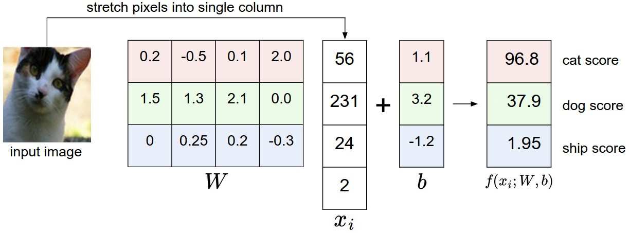
Fig. 5.2 Linear perceptron for images. The output is the logit score. Source http://cs231n.github.io/linear-classify

The net activations form a vector \(\mathbf{z}\):

\[ \mathbf{z} = f_{W, \mathbf{b}}(\mathbf{x}) = W \times \mathbf{x} + \mathbf{b} \]

Each element \(z_j\) of the vector \(\mathbf{z}\) is called the logit score of the class: the higher the score, the more likely the input belongs to this class. The logit scores are not probabilities, as they can be negative and do not sum to 1.

5.2.1. One-hot encoding

How do we represent the ground truth \(\mathbf{t}\) for each neuron? The target vector \(\mathbf{t}\) is represented using one-hot encoding. The binary vector has one element per class: only one element is 1, the others are 0. Example:

\[ \mathbf{t} = [\text{cat}, \text{dog}, \text{ship}, \text{house}, \text{car}] = [0, 1, 0, 0, 0] \]

The labels can be seen as a probability distribution over the training set, in this case a multinomial distribution (a dice with \(C\) sides). For a given image \(\mathbf{x}\) (e.g. a picture of a dog), the conditional pmf is defined by the one-hot encoded vector \(\mathbf{t}\):

\[P(\mathbf{t} | \mathbf{x}) = [P(\text{cat}| \mathbf{x}), P(\text{dog}| \mathbf{x}), P(\text{ship}| \mathbf{x}), P(\text{house}| \mathbf{x}), P(\text{car}| \mathbf{x})] = [0, 1, 0, 0, 0]\]

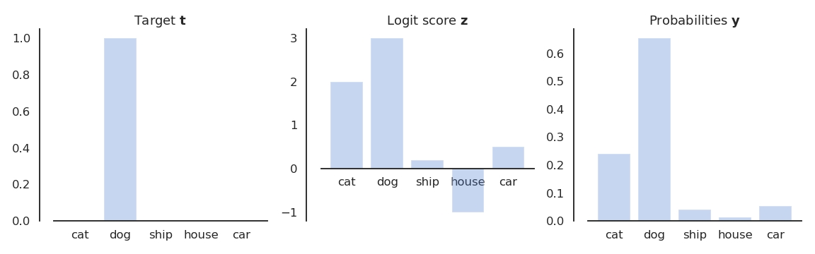
Fig. 5.3 The logit scores \(\mathbf{z}\) cannot be compared to the targets \(\mathbf{t}\): we need to transform them into a probability distribution \(\mathbf{y}\).

We need to transform the logit score \(\mathbf{z}\) into a probability distribution \(P(\mathbf{y} | \mathbf{x})\) that should be as close as possible from \(P(\mathbf{t} | \mathbf{x})\).

5.2.2. Softmax activation

The softmax operator makes sure that the sum of the outputs \(\mathbf{y} = \{y_i\}\) over all classes is 1.

\[ y_j = P(\text{class = j} | \mathbf{x}) = \mathcal{S}(z_j) = \frac{\exp(z_j)}{\sum_k \exp(z_k)} \]

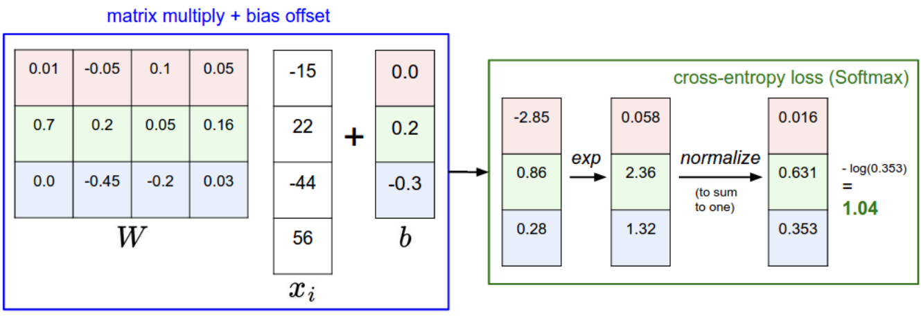
Fig. 5.4 Softmax activation transforms the logit score into a probability distribution. Source http://cs231n.github.io/linear-classify

The higher \(z_j\), the higher the probability that the example belongs to class \(j\). This is very similar to logistic regression for soft classification, except that we have multiple classes.

5.2.3. Cross-entropy loss function

We cannot use the mse as a loss function, as the softmax function would be hard to differentiate:

\[ \text{mse}(W, \mathbf{b}) = \sum_j (t_{j} - \frac{\exp(z_j)}{\sum_k \exp(z_k)})^2 \]

We actually want to minimize the statistical distance netween two distributions:

• The model outputs a multinomial probability distribution \(\mathbf{y}\) for an input \(\mathbf{x}\): \(P(\mathbf{y} | \mathbf{x}; W, \mathbf{b})\).

• The one-hot encoded classes also come from a multinomial probability distribution \(P(\mathbf{t} | \mathbf{x})\).

We search which parameters \((W, \mathbf{b})\) make the two distributions \(P(\mathbf{y} | \mathbf{x}; W, \mathbf{b})\) and \(P(\mathbf{t} | \mathbf{x})\) close. The training data \(\{\mathbf{x}_i, \mathbf{t}_i\}\) represents samples from \(P(\mathbf{t} | \mathbf{x})\). \(P(\mathbf{y} | \mathbf{x}; W, \mathbf{b})\) is a good model of the data when the two distributions are close, i.e. when the negative log-likelihood of each sample under the model is small.

Fig. 5.5 Cross-entropy between two distributions \(X\) and \(Y\): are samples of \(X\) likely under \(Y\)?

For an input \(\mathbf{x}\), we minimize the cross-entropy between the target distribution and the predicted outputs:

\[ \mathcal{l}(W, \mathbf{b}) = \mathcal{H}(\mathbf{t} | \mathbf{x}, \mathbf{y} | \mathbf{x}) = \mathbb{E}_{t \sim P(\mathbf{t} | \mathbf{x})} [ - \log P(\mathbf{y} = t | \mathbf{x})] \]

The cross-entropy samples from \(\mathbf{t} | \mathbf{x}\):

\[ \mathcal{l}(W, \mathbf{b}) = \mathcal{H}(\mathbf{t} | \mathbf{x}, \mathbf{y} | \mathbf{x}) = \mathbb{E}_{t \sim P(\mathbf{t} | \mathbf{x})} [ - \log P(\mathbf{y} = t | \mathbf{x})] \]

For a given input \(\mathbf{x}\), \(\mathbf{t}\) is non-zero only for the correct class \(t^*\), as \(\mathbf{t}\) is a one-hot encoded vector \([0, 1, 0, 0, 0]\):

\[ \mathcal{l}(W, \mathbf{b}) = - \log P(\mathbf{y} = t^* | \mathbf{x}) \]

If we note \(j^*\) the index of the correct class \(t^*\), the cross entropy is simply:

\[ \mathcal{l}(W, \mathbf{b}) = - \log y_{j^*} \]

As only one element of \(\mathbf{t}\) is non-zero, the cross-entropy is the same as the negative log-likelihood of the prediction for the true label:

\[ \mathcal{l}(W, \mathbf{b}) = - \log y_{j^*} \]

The minimum of \(- \log y\) is obtained when \(y =1\): We want to classifier to output a probability 1 for the true label. Because of the softmax activation function, the probability for the other classes should become closer from 0.

\[ y_j = P(\text{class = j}) = \frac{\exp(z_j)}{\sum_k \exp(z_k)} \]

Minimizing the cross-entropy / negative log-likelihood pushes the output distribution \(\mathbf{y} | \mathbf{x}\) to be as close as possible to the target distribution \(\mathbf{t} | \mathbf{x}\).

Fig. 5.6 Minimizing the cross-entropy between \(\mathbf{t} | \mathbf{x}\) and \(\mathbf{y} | \mathbf{x}\) makes them similar.

As \(\mathbf{t}\) is a binary vector \([0, 1, 0, 0, 0]\), the cross-entropy / negative log-likelihood can also be noted as the dot product between \(\mathbf{t}\) and \(\log \mathbf{y}\):

\[ \mathcal{l}(W, \mathbf{b}) = - \langle \mathbf{t} \cdot \log \mathbf{y} \rangle = - \sum_{j=1}^C t_j \, \log y_j = - \log y_{j^*} \]

The cross-entropy loss function is then the expectation over the training set of the individual cross-entropies:

\[ \mathcal{L}(W, \mathbf{b}) = \mathbb{E}_{\mathbf{x}, \mathbf{t} \sim \mathcal{D}} [- \langle \mathbf{t} \cdot \log \mathbf{y} \rangle ] \approx \frac{1}{N} \sum_{i=1}^N - \langle \mathbf{t}_i \cdot \log \mathbf{y}_i \rangle \]

The nice thing with the cross-entropy loss function, when used on a softmax activation function, is that the partial derivative w.r.t the logit score \(\mathbf{z}\) is simple:

\[\begin{split} \begin{split} \frac{\partial {l}(W, \mathbf{b})}{\partial z_i} & = - \sum_j \frac{\partial}{\partial z_i} t_j \log(y_j)= - \sum_j t_j \frac{\partial \log(y_j)}{\partial z_i} = - \sum_j t_j \frac{1}{y_j} \frac{\partial y_j}{\partial z_i} \\ & = - \frac{t_i}{y_i} \frac{\partial y_i}{\partial z_i} - \sum_{j \neq i}^C \frac{t_j}{y_j} \frac{\partial y_j}{\partial z_i} = - \frac{t_i}{y_i} y_i (1-y_i) - \sum_{j \neq i}^C \frac{t_j}{y_i} (-y_j \, y_i) \\ & = - t_i + t_i \, y_i + \sum_{j \neq i}^C t_j \, y_i = - t_i + \sum_{j = 1}^C t_j y_i = -t_i + y_i \sum_{j = 1}^C t_j \\ & = - (t_i - y_i) \end{split} \end{split}\]

i.e. the same as with the mse in linear regression! Refer https://peterroelants.github.io/posts/cross-entropy-softmax/ for more explanations on the proof.

Note

When differentiating a softmax probability \(y_j = \dfrac{\exp(z_j)}{\sum_k \exp(z_k)}\) w.r.t a logit score \(z_i\), i.e. \(\dfrac{\partial y_j}{\partial z_i}\), we need to consider two cases:

• If \(i=j\), \(\exp(z_i)\) appears both at the numerator and denominator of \(\frac{\exp(z_i)}{\sum_k \exp(z_k)}\). The product rule \((f\times g)' = f'\, g + f \, g'\) gives us:

\[\begin{split}\begin{aligned} \dfrac{\partial \log(y_i)}{\partial z_i} &= \dfrac{\exp(z_i)}{\sum_k \exp(z_k)} + \exp(z_i) \, \dfrac{- \exp(z_i)}{(\sum_k \exp(z_k))^2} \\ &= \dfrac{\exp(z_i) \, \sum_k \exp(z_k) - \exp(z_i)^2}{(\sum_k \exp(z_k))^2} \\ &= \dfrac{\exp(z_i)}{\sum_k \exp(z_k)} \, (1- \dfrac{\exp(z_i)}{\sum_k \exp(z_k)})\\ &= y_i \, (1 - y_i)\\ \end{aligned} \end{split}\]

This is similar to the derivative of the logistic function.

• If \(i \neq j\), \(z_i\) only appears at the denominator, so we only need the chain rule:

\[\begin{split}\begin{aligned} \dfrac{\partial \log(y_j)}{\partial z_i} &= - \exp(z_j) \, \dfrac{\exp(z_i)}{(\sum_k \exp(z_k))^2} \\ &= - \dfrac{\exp(z_i)}{\sum_k \exp(z_k)} \, \dfrac{\exp(z_j)}{\sum_k \exp(z_k)} \\ &= - y_i \, y_j \\ \end{aligned} \end{split}\]

Using the vector notation, we get:

\[ \frac{\partial \mathcal{l}(W, \mathbf{b})}{\partial \mathbf{z}} = - (\mathbf{t} - \mathbf{y} ) \]

As:

\[ \mathbf{z} = W \times \mathbf{x} + \mathbf{b} \]

we can obtain the partial derivatives:

\[\begin{split} \begin{cases} \dfrac{\partial \mathcal{l}(W, \mathbf{b})}{\partial W} = \dfrac{\partial \mathcal{l}(W, \mathbf{b})}{\partial \mathbf{z}} \times \dfrac{\partial \mathbf{z}}{\partial W} = - (\mathbf{t} - \mathbf{y} ) \times \mathbf{x}^T \\ \\ \dfrac{\partial \mathcal{l}(W, \mathbf{b})}{\partial \mathbf{b}} = \dfrac{\partial \mathcal{l}(W, \mathbf{b})}{\partial \mathbf{z}} \times \dfrac{\partial \mathbf{z}}{\partial \mathbf{b}} = - (\mathbf{t} - \mathbf{y} ) \\ \end{cases} \end{split}\]

So gradient descent leads to the delta learning rule:

\[\begin{split} \begin{cases} \Delta W = \eta \, (\mathbf{t} - \mathbf{y} ) \times \mathbf{x}^T \\ \\ \Delta \mathbf{b} = \eta \, (\mathbf{t} - \mathbf{y} ) \\ \end{cases} \end{split}\]

Softmax linear classifier

• We first compute the logit scores \(\mathbf{z}\) using a linear layer:

\[ \mathbf{z} = W \times \mathbf{x} + \mathbf{b} \]

• We turn them into probabilities \(\mathbf{y}\) using the softmax activation function:

\[ y_j = \frac{\exp(z_j)}{\sum_k \exp(z_k)} \]

• We minimize the cross-entropy / negative log-likelihood on the training set:

\[ \mathcal{L}(W, \mathbf{b}) = \mathbb{E}_{\mathbf{x}, \mathbf{t} \sim \mathcal{D}} [ - \langle \mathbf{t} \cdot \log \mathbf{y} \rangle] \]

which simplifies into the delta learning rule:

\[\begin{split} \begin{cases} \Delta W = \eta \, (\mathbf{t} - \mathbf{y} ) \times \mathbf{x}^T \\ \\ \Delta \mathbf{b} = \eta \, (\mathbf{t} - \mathbf{y} ) \\ \end{cases} \end{split}\]

5.2.4. Comparison of linear classification and regression

Classification and regression differ in the nature of their outputs: in classification they are discrete, in regression they are continuous values. However, when trying to minimize the mismatch between a model \(\mathbf{y}\) and the real data \(\mathbf{t}\), we have found the same delta learning rule:

\[\begin{split} \begin{cases} \Delta W = \eta \, (\mathbf{t} - \mathbf{y} ) \times \mathbf{x}^T \\ \\ \Delta \mathbf{b} = \eta \, (\mathbf{t} - \mathbf{y} ) \\ \end{cases} \end{split}\]

Regression and classification are in the end the same problem for us. The only things that needs to be adapted is the activation function of the output and the loss function:

• For regression, we use regular activation functions and the mean square error (mse):

  \[ \mathcal{L}(W, \mathbf{b}) = \mathbb{E}_{\mathbf{x}, \mathbf{t} \in \mathcal{D}} [ ||\mathbf{t} - \mathbf{y}||^2 ] \]

• For classification, we use the softmax activation function and the cross-entropy (negative log-likelihood) loss function:

  \[\mathcal{L}(W, \mathbf{b}) = \mathbb{E}_{\mathbf{x}, \mathbf{t} \sim \mathcal{D}} [ - \langle \mathbf{t} \cdot \log \mathbf{y} \rangle]\]

5.3. Multi-label classification

What if there is more than one label on the image? The target vector \(\mathbf{t}\) does not represent a probability distribution anymore:

\[ \mathbf{t} = [\text{cat}, \text{dog}, \text{ship}, \text{house}, \text{car}] = [1, 1, 0, 0, 0] \]

Normalizing the vector does not help: it is not a dog or a cat, it is a dog and a cat.

\[ \mathbf{t} = [\text{cat}, \text{dog}, \text{ship}, \text{house}, \text{car}] = [0.5, 0.5, 0, 0, 0] \]

For multi-label classification, we can simply use the logistic activation function for the output neurons:

\[ \mathbf{y} = \sigma(W \times \mathbf{x} + \mathbf{b}) \]

The outputs are between 0 and 1, but they do not sum to one. Each output neuron performs a logistic regression for soft classification on their class:

\[y_j = P(\text{class} = j | \mathbf{x})\]

Each output neuron \(y_j\) has a binary target \(t_j\) (one-vs-the-rest) and has to minimize the negative log-likelihood:

\[ \mathcal{l}_j(W, \mathbf{b}) = - t_j \, \log y_j + (1 - t_j) \, \log( 1- y_j) \]

The binary cross-entropy loss for the whole network is the sum of the negative log-likelihood for each class:

\[ \mathcal{L}(W, \mathbf{b}) = \mathbb{E}_{\mathcal{D}} [- \sum_{j=1}^C t_j \, \log y_j + (1 - t_j) \, \log( 1- y_j)] \]

previous

4. Linear classification

next

6. Learning theory