
4.1. Multiple linear regression
Let’s now investigate multiple linear regression (MLR), where several output depends on more than one input variable:
The Boston Housing Dataset consists of price of houses in various places in Boston. Alongside with price, the dataset also provide information such as the crime rate (CRIM), the proportion of non-retail business acres per town (INDUS), the proportion of owner-occupied units built prior to 1940 (AGE) and several other attributes. It is available here : https://archive.ics.uci.edu/ml/machine-learning-databases/housing.
The Boston dataset can be directly downloaded from scikit-learn:
import numpy as np
import matplotlib.pyplot as plt

from sklearn.datasets import load_boston

boston = load_boston()

X = boston.data
t = boston.target

print(X.shape)
print(t.shape)
(506, 13)
(506,)
There are 506 samples with 13 inputs and one output (the price). The following cell decribes what the features are:
print(boston.DESCR)
.. _boston_dataset:

Boston house prices dataset
---------------------------

**Data Set Characteristics:**

    :Number of Instances: 506

    :Number of Attributes: 13 numeric/categorical predictive. Median Value (attribute 14) is usually the target.

    :Attribute Information (in order):
        - CRIM     per capita crime rate by town
        - ZN       proportion of residential land zoned for lots over 25,000 sq.ft.
        - INDUS    proportion of non-retail business acres per town
        - CHAS     Charles River dummy variable (= 1 if tract bounds river; 0 otherwise)
        - NOX      nitric oxides concentration (parts per 10 million)
        - RM       average number of rooms per dwelling
        - AGE      proportion of owner-occupied units built prior to 1940
        - DIS      weighted distances to five Boston employment centres
        - RAD      index of accessibility to radial highways
        - TAX      full-value property-tax rate per $10,000
        - PTRATIO  pupil-teacher ratio by town
        - B        1000(Bk - 0.63)^2 where Bk is the proportion of blacks by town
        - LSTAT    % lower status of the population
        - MEDV     Median value of owner-occupied homes in $1000's

    :Missing Attribute Values: None

    :Creator: Harrison, D. and Rubinfeld, D.L.

This is a copy of UCI ML housing dataset.
https://archive.ics.uci.edu/ml/machine-learning-databases/housing/


This dataset was taken from the StatLib library which is maintained at Carnegie Mellon University.

The Boston house-price data of Harrison, D. and Rubinfeld, D.L. 'Hedonic
prices and the demand for clean air', J. Environ. Economics & Management,
vol.5, 81-102, 1978.   Used in Belsley, Kuh & Welsch, 'Regression diagnostics
...', Wiley, 1980.   N.B. Various transformations are used in the table on
pages 244-261 of the latter.

The Boston house-price data has been used in many machine learning papers that address regression
problems.

.. topic:: References

   - Belsley, Kuh & Welsch, 'Regression diagnostics: Identifying Influential Data and Sources of Collinearity', Wiley, 1980. 244-261.
   - Quinlan,R. (1993). Combining Instance-Based and Model-Based Learning. In Proceedings on the Tenth International Conference of Machine Learning, 236-243, University of Massachusetts, Amherst. Morgan Kaufmann.
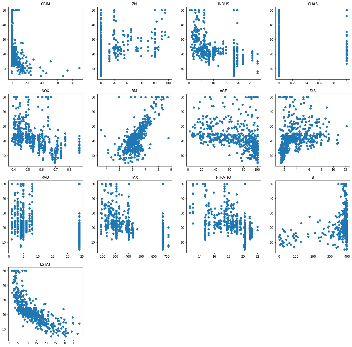
The following cell allows to visualize how each feature influences the price individually:
plt.figure(figsize=(20, 20))

for i in range(13):
    plt.subplot(4, 4 , i+1)
    plt.scatter(X[:, i], t)
    plt.title(boston.feature_names[i])
plt.show()
4.1.1. Linear regression
Q: Apply MLR on the Boston data using the same LinearRegression method of scikit-learn as last time. Print the mse and visualize the prediction \(y\) against the true value \(t\) for each sample as before. Does it work?
You will also plot the weights of the model (reg.coef_) and conclude on the relative importance of the different features: which feature has the stronger weight and why?
A good practice in machine learning is to normalize the inputs, i.e. to make sure that the samples have a mean of 0 and a standard deviation of 1. scikit-learn provides a method named scale that does it automatically:
from sklearn.preprocessing import scale

X_scaled = scale(X)
Q: Apply MLR again on X_scaled, print the mse and visualize the weights. What has changed?
4.1.2. Regularized regression
Now is time to investigate regularization:
MLR with L2 regularization is called Ridge regression
MLR with L1 regularization is called Lasso regression
Fortunately, scikit-learn provides these methods with a similar interface to LinearRegression. The Ridge and Lasso objects take an additional argument alpha which represents the regularization parameter:
reg = Ridge(alpha=0.1)
reg = Lasso(alpha=0.1)
from sklearn.linear_model import Ridge, Lasso
Q: Apply Ridge and Lasso regression on the scaled data, vary the regularization parameter to understand its function and comment on the results. In particular, increase the regularization parameter for LASSO and identify the features which are the most predictive of the price. Does it make sense?