
2. Hopfield networks
Slides: pdf
2.1. Associative memory
In deep learning, our biggest enemy was overfitting, i.e. learning by heart the training examples. But what if it was actually useful in cognitive tasks? Deep networks implement a procedural memory: they know how to do things. A fundamental aspect of cognition is episodic memory: remembering when specific events happened.
Fig. 2.57 Hierarchy of memories. Source: https://brain-basedlearning.weebly.com/memory.html
Episodic memory is particularly useful when retrieving memories from degraded or partial inputs. When the reconstruction is similar to the remembered input, we talk about auto-associative memory. An item can be retrieved by just knowing part of its content: content-adressable memory.
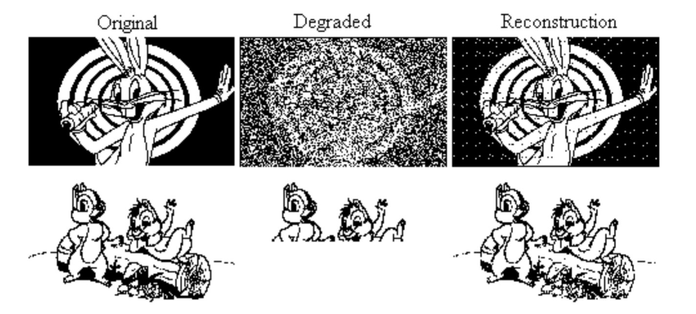
Fig. 2.58 Content-adressable memory. Source: https://www.cs.cmu.edu/~bhiksha/courses/deeplearning/Fall.2015/slides/lec14.hopfield.pdf
Auto-associative memory
Hmunas rmebmeer iamprtnot envtes in tiher leivs. You mihgt be albe to rlecal eervy deiatl of yuor frist eaxm at cllgeoe; or of yuor fsirt pbuilc sepceh; or of yuor frsit day in katigrneedrn; or the fisrt tmie you wnet to a new scohol atefr yuor fimlay mveod to a new ctiy. Hmaun moemry wkors wtih asncisoatois. If you haer the vicoe of an old fernid on the pnohe, you may slntesnoauopy rlaecl seortis taht you had not tghuoht of for yares. If you are hrgnuy and see a pcturie of a bnaana, you mihgt vdivliy rclael the ttsae and semll of a bnanaa and teerbhy rieazle taht you are ideend hngury. In tihs lcterue, we peesrnt modles of nrueal ntkweros taht dbriecse the rcaell of puielovsry seortd imtes form mmorey.
Text scrambler by http://www.stevesachs.com/jumbler.cgi
The classical approach to auto-associative memrories is the nearest neighbour algorithm (KNN). One compares a new input to each of the training examples using a given metric (distance) and assigns the input to the closest example.
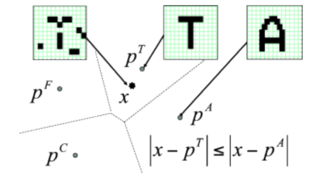
Fig. 2.59 Nearest neighbour algorithm. Source: http://didawiki.di.unipi.it/lib/exe/fetch.php/bionics-engineering/computational-neuroscience/2-hopfield-hand.pdf
Another approach is to have a recurrent neural network memorize the training examples and retrieve them given the input.
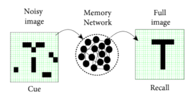
Fig. 2.60 Neural associative memory. Source: http://didawiki.di.unipi.it/lib/exe/fetch.php/bionics-engineering/computational-neuroscience/2-hopfield-hand.pdf
When the reconstruction is different from the input, it is an hetero-associative memory. Hetero-associative memories often work in both directions (bidirectional associative memory), e.g. name \(\leftrightarrow\) face.
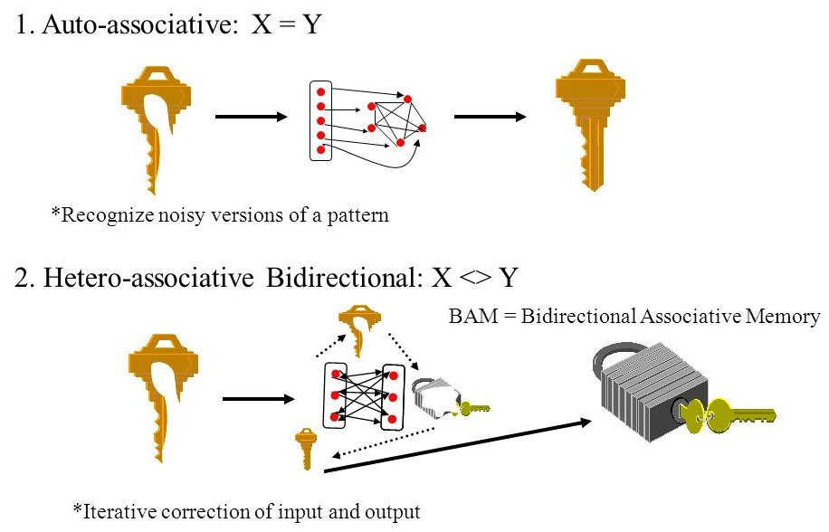
Fig. 2.61 Hetero-associative memory. Source: https://slideplayer.com/slide/7303074/
2.2. Hopfield networks
2.2.1. Structure
Feedforward networks only depend on the current input:
Recurrent networks also depend on their previous output:
Both are strongly dependent on their inputs and do not have their own dynamics.
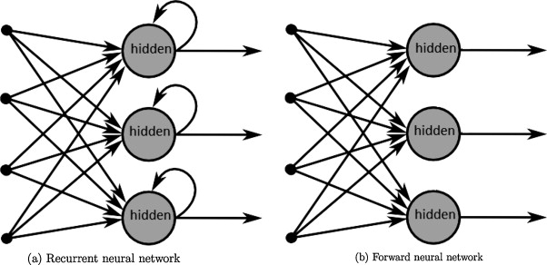
Fig. 2.62 Feedforward networks and RNN have no dynamics. Source: https://www.researchgate.net/publication/266204519_A_Survey_on_the_Application_of_Recurrent_Neural_Networks_to_Statistical_Language_Modeling
Hopfield networks [Hopfield, 1982] only depend on a single input (one constant value per neuron) and their previous output using recurrent weights:
For a single constant input \(\mathbf{x}\), one lets the network converge for enough time steps \(T\) and observe what the final output \(\mathbf{y}_T\) is.
Hopfield network have their own dynamics: the output evolves over time, but the input is constant. One can even omit the input \(\mathbf{x}\) and merge it with the bias \(\mathbf{b}\): the dynamics will only depend on the initial state \(\mathbf{y}_0\).
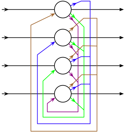
Fig. 2.63 Hopfield network. Source: https://en.wikipedia.org/wiki/Hopfield_network
Binary Hopfield networks use binary units. The neuron \(i\) has a net activation \(x_i\) (potential) depending on the other neurons \(j\) through weights \(w_{ji}\):
The output \(y_i\) is the sign of the potential:
There are no self-connections: \(w_{ii} = 0\). The weights are symmetrical: \(w_{ij} = w_{ji}\).
In matrix-vector form:
2.2.2. Asynchronous evaluation
At each time step, a neuron will flip its state if the sign of the potential \(x_i = \sum_{j \neq i} w_{ji} \, y_j + b\) does not match its current output \(y_i\). This will in turn modify the potential of all other neurons, who may also flip. The potential of that neuron may change its sign, so the neuron will flip again. After a finite number of iterations, the network reaches a stable state (proof later). Neurons are evaluated one after the other: asynchronous evaluation.
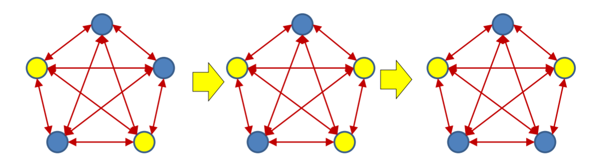
Fig. 2.64 Asynchronous evaluation. Source: https://www.cs.cmu.edu/~bhiksha/courses/deeplearning/Fall.2015/slides/lec14.hopfield.pdf
Let’s consider a Hopfield network with 5 neurons, sparse connectivity and no bias. In the initial state, 2 neurons are on (+1), 3 are off (-1).

Let’s evaluate the top-right neuron. Its potential is -4 * 1 + 3 * (-1) + 3 * (-1) = -10 \(<\) 0. Its output stays at -1.
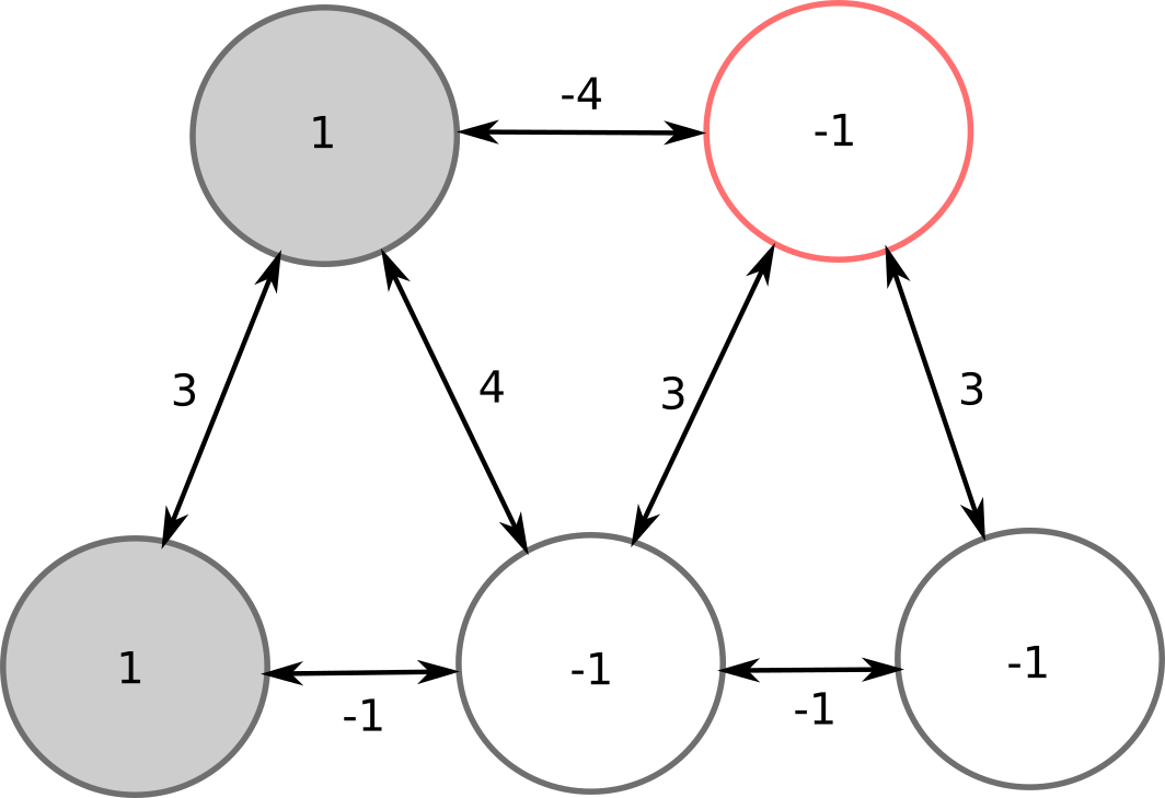
Now the bottom-left neuron: 3 * 1 + (-1) * (-1) = 4 \(>\) 0, the output stays at +1.
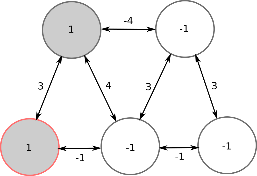
But the bottom-middle neuron has to flip its sign: -1 * 1 + 4 * 1 + 3 * (-1) - 1 * (-1) = 1 \(>\) 0. Its new output is +1.
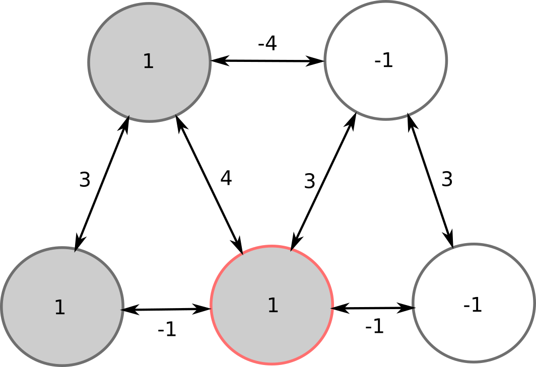
We can continue evaluating the neurons, but nobody will flip its sign. This configuration is a stable pattern of the network.

There is another stable pattern, where the two other neurons are active: symmetric or ghost pattern. All other patterns are unstable and will eventually lead to one of the two stored patterns.

2.2.3. Hopfield network
The weight matrix \(W\) allows to encode a given number of stable patterns, which are fixed points of the network’s dynamics. Any initial configuration will converge to one of the stable patterns.
Algorithm
Initialize a symmetrical weight matrix without self-connections.
Set an input to the network through the bias \(\mathbf{b}\).
while not stable:
Pick a neuron \(i\) randomly.
Compute its potential:
\[x_i = \sum_{j \neq i} w_{ji} \, y_j + b\]Flip its output if needed:
\[y_i = \text{sign}(x_i)\]
Why do we need to update neurons one by one, instead of all together as in ANNs (vector-based)? Consider the two neurons below:

If you update them at the same time, they will both flip:

But at the next update, they will both flip again: the network will oscillate for ever.
By updating neurons one at a time (randomly), you make sure that the network converges to a stable pattern:

2.2.4. Energy of the Hopfield network
Let’s have a look at the quantity \(y_i \, (\sum_{j \neq i} w_{ji} \, y_j + b)\) before and after an update:
If the neuron does not flip, the quantity does not change.
If the neuron flips (\(y_i\) goes from +1 to -1, or from -1 to +1), this means that:
\(y_i\) and \(\sum_{j \neq i} w_{ji} \, y_j + b\) had different signs before the update, so \(y_i \, (\sum_{j \neq i} w_{ji} \, y_j + b)\) was negative.
After the flip, \(y_i\) and \(\sum_{j \neq i} w_{ji} \, y_j + b\) have the same sign, so \(y_i \, (\sum_{j \neq i} w_{ji} \, y_j + b)\) becomes positive.
The change in the quantity \(y_i \, (\sum_{j \neq i} w_{ji} \, y_j + b)\) is always positive or equal to zero:
No update can decrease this quantity.
Let’s now sum this quantity over the complete network and reverse its sign:
We can expand it and simplify it knowing that \(w_{ii}=0\) and \(w_{ij} = w_{ji}\):
The term \(\frac{1}{2}\) comes from the fact that the weights are symmetric and count twice in the double sum.
In a matrix-vector form, it becomes:
\(E(\mathbf{y})\) is called the energy of the network or its Lyapunov function for a pattern \((\mathbf{y})\). We know that updates can only decrease the energy of the network, it will never go up. Moreover, the energy has a lower bound: it cannot get below a certain value as everything is finite.
Stable patterns are local minima of the energy function: no update can increase the energy.
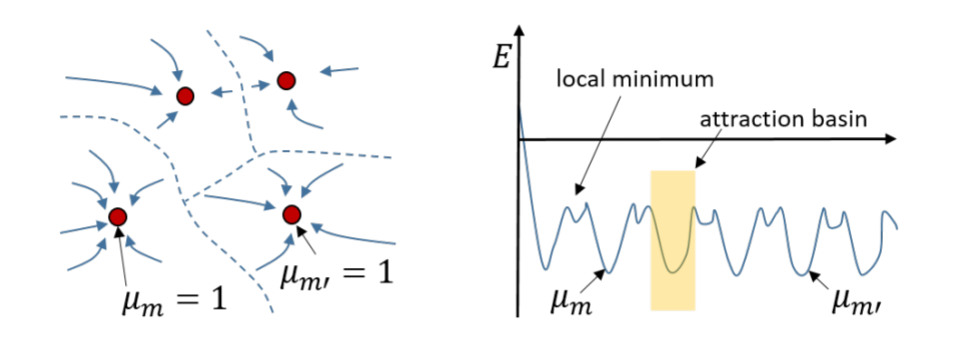
Fig. 2.65 The energy landscape has several local minima. All states within the attraction basin converge to the point attractor. Source: http://didawiki.di.unipi.it/lib/exe/fetch.php/bionics-engineering/computational-neuroscience/2-hopfield-hand.pdf
Stable patterns are also called point attractors. Other patterns have higher energies and are attracted by the closest stable pattern (attraction basin).
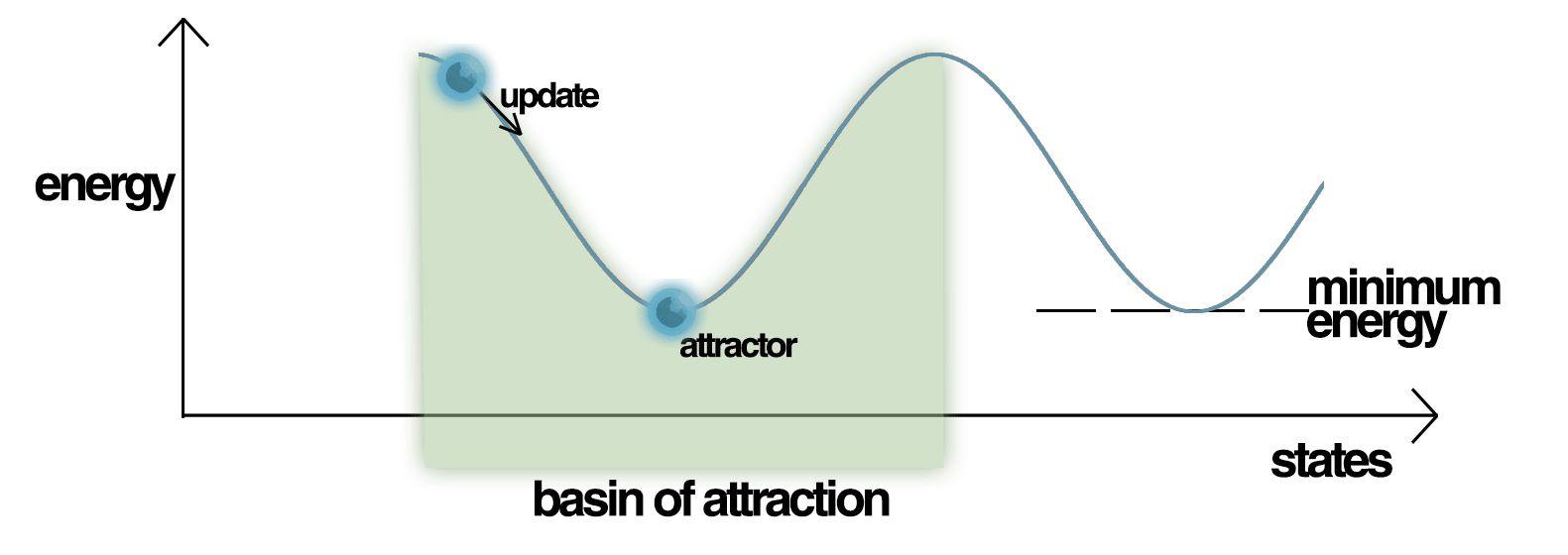
Fig. 2.66 Energy landscape. Source: https://en.wikipedia.org/wiki/Hopfield_network
It can be shown [McEliece et al., 1987] that for a network with \(N\) units, one can store up to \(0.14 N\) different patterns:
If you have 1000 neurons, you can store 140 patterns. As you need 1 million weights for it, it is not very efficient…
2.2.5. Storing patterns with Hebbian learning
The weights define the stored patterns through their contribution to the energy:
How do you choose the weights \(W\) so that the desired patterns \((\mathbf{y}^1, \mathbf{y}^2, \dots, \mathbf{y}^P)\) are local minima of the energy function?
Let’s omit the bias for a while, as it does not depend on \(W\). One can replace the bias with a weight to a neuron whose activity is always +1. The pattern \(\mathbf{y}^1 = [y^1_1, y^1_2, \ldots, y^1_N]^T\) is stable if no neuron flips after the update:
Which weights respect this stability constraint?
Hebb’s rule: Cells that fire together wire together
When an axon of cell A is near enough to excite a cell B and repeatedly or persistently takes part in firing it, some growth process or metabolic change takes place in one or both cells such that A’s efficiency, as one of the cells firing B, is increased.
Donald Hebb, 1949
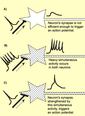
Fig. 2.67 Hebb’s rule. Source: https://thebrain.mcgill.ca/flash/i/i_07/i_07_cl/i_07_cl_tra/i_07_cl_tra.html
Hebbian learning between two neurons states that the synaptic efficiency (weight) of their connection should be increased if the activity of the two neurons is correlated. The correlation between the activities is simply the product:
If both activities are high, the weight will increase. If one of the activities is low, the weight won’t change. It is a very rudimentary model of synaptic plasticity, but verified experimentally.
The fixed point respects:
If we use \(w_{i,j} = y^1_i \, y^1_j\) as the result of Hebbian learning (weights initialized at 0), we obtain
as \(y^1_j \, y^1_j = 1\) (binary units). This means that setting \(w_{i,j} = y^1_i \, y^1_j\) makes \(\mathbf{y}^1\) a fixed point of the system! Remembering that \(w_{ii}=0\), we find that \(W\) is the correlation matrix of \(\mathbf{y}^1\) minus the identity:
(the diagonal of \(\mathbf{y}^1 \times (\mathbf{y}^1)^T\) is always 1, as \(y^1_j \, y^1_j = 1\)).
If we have \(P\) patterns \((\mathbf{y}^1, \mathbf{y}^2, \dots, \mathbf{y}^P)\) to store, the corresponding weight matrix is:
\(\frac{1}{P} \, \sum_{k=1}^P \mathbf{y}^k \times (\mathbf{y}^k)^T\) is the correlation matrix of the patterns.
This does not sound much like learning as before, as we are forming the matrix directly from the data, but it is a biologically realistic implementation of Hebbian learning. We only need to iterate once over the training patterns, not multiple epochs. Learning can be online: the weight matrix is modified when a new pattern \(\mathbf{y}^k\) has to be remembered:
There is no catastrophic forgetting until we reach the capacity \(C = 0.14 \, N\) of the network.
Storing patterns in an Hopfield network
Given \(P\) patterns \((\mathbf{y}^1, \mathbf{y}^2, \dots, \mathbf{y}^P)\) to store, build the weight matrix:
The energy of the Hopfield network for a new pattern \(\mathbf{y}\) is (implicitly):
i.e. a quadratic function of the dot product between the current pattern \(\mathbf{y}\) and the stored patterns \(\mathbf{y}^k\).
The stored patterns are local minima of this energy function, which can be retrieved from any pattern \(\mathbf{y}\) by iteratively applying the asynchronous update:
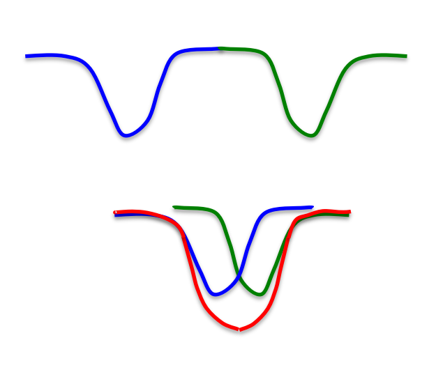
Fig. 2.68 Spurious patterns. Source: https://www.cs.cmu.edu/~bhiksha/courses/deeplearning/Fall.2015/slides/lec14.hopfield.pdf
The problem when the capacity of the network is full is that the stored patterns will start to overlap. The retrieved patterns will be a linear combination of the stored patterns, what is called a spurious pattern or metastable state.
A spurious pattern has never seen by the network, but is remembered like other memories (hallucinations).
Unlearning methods [Hopfield et al., 1983] use a sleep / wake cycle:
When the network is awake, it remembers patterns.
When the network sleeps (dreams), it unlearns spurious patterns.
2.2.6. Applications of Hopfield networks
Optimization:
Traveling salesman problem http://fuzzy.cs.ovgu.de/ci/nn/v07_hopfield_en.pdf
Timetable scheduling
Routing in communication networks
Physics:
Spin glasses (magnetism)
Computer Vision:
Image reconstruction and restoration
Neuroscience:
Models of the hippocampus, episodic memory
2.3. Modern Hopfield networks / Dense Associative Memories (optional)
The problems with Hopfield networks are:
Their limited capacity \(0.14 \, N\).
Ghost patterns (reversed images).
Spurious patterns (bad separation of patterns).
Retrieval is not error-free.
In this example, the masked Homer is closer to the Bart pattern in the energy function, so it converges to its ghost pattern.
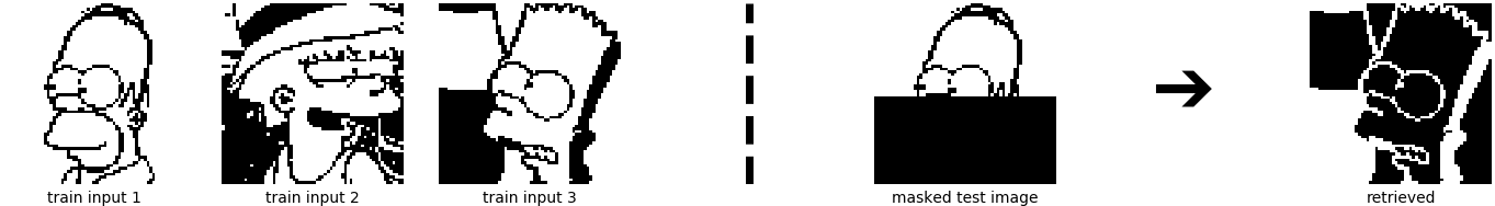
Fig. 2.69 Retrieval error with old-school Hopfield networks. Source: https://ml-jku.github.io/hopfield-layers/
The problem comes mainly from the fact the energy function is a quadratic function of the dot product between a state \(\mathbf{y}\) and the patterns \(\mathbf{y}^k\):
\(-((\mathbf{y}^k)^T \times \mathbf{y})^2\) has minimum when \(\mathbf{y} = \mathbf{y}^k\). Quadratic functions are very wide, so it is hard to avoid overlap between the patterns. If we had a sharper energy functions, could not we store more patterns and avoid interference?
Yes. We could define the energy function as a polynomial function of order \(a> 2\) [Krotov & Hopfield, 2016]:
and get a polynomial capacity \(C \approx \alpha_a \, N^{a-1}\). Or even an exponential function \(a = \infty\) [Demircigil et al., 2017]:
and get an exponential capacity \(C \approx 2^{\frac{N}{2}}\)! One could store exponentially more patterns than neurons. The question is then: which update rule would minimize these energies?
[Krotov & Hopfield, 2016] and [Demircigil et al., 2017] show that the binary units \(y_i\) can still be updated asynchronously by comparing the energy of the model with the unit on or off:
If the energy is lower with the unit on than with the unit off, turn it on! Otherwise turn it off. Note that computing the energy necessitates to iterate over all patterns, so in practice you should keep the number of patterns small:
However, you are not bounded by \(0.14 \, N\) anymore, just by the available computational power and RAM.
The increased capacity of the modern Hopfield network makes sure that you store many patterns without interference (separability of patterns). Convergence occurs in only one step (one update per neuron).
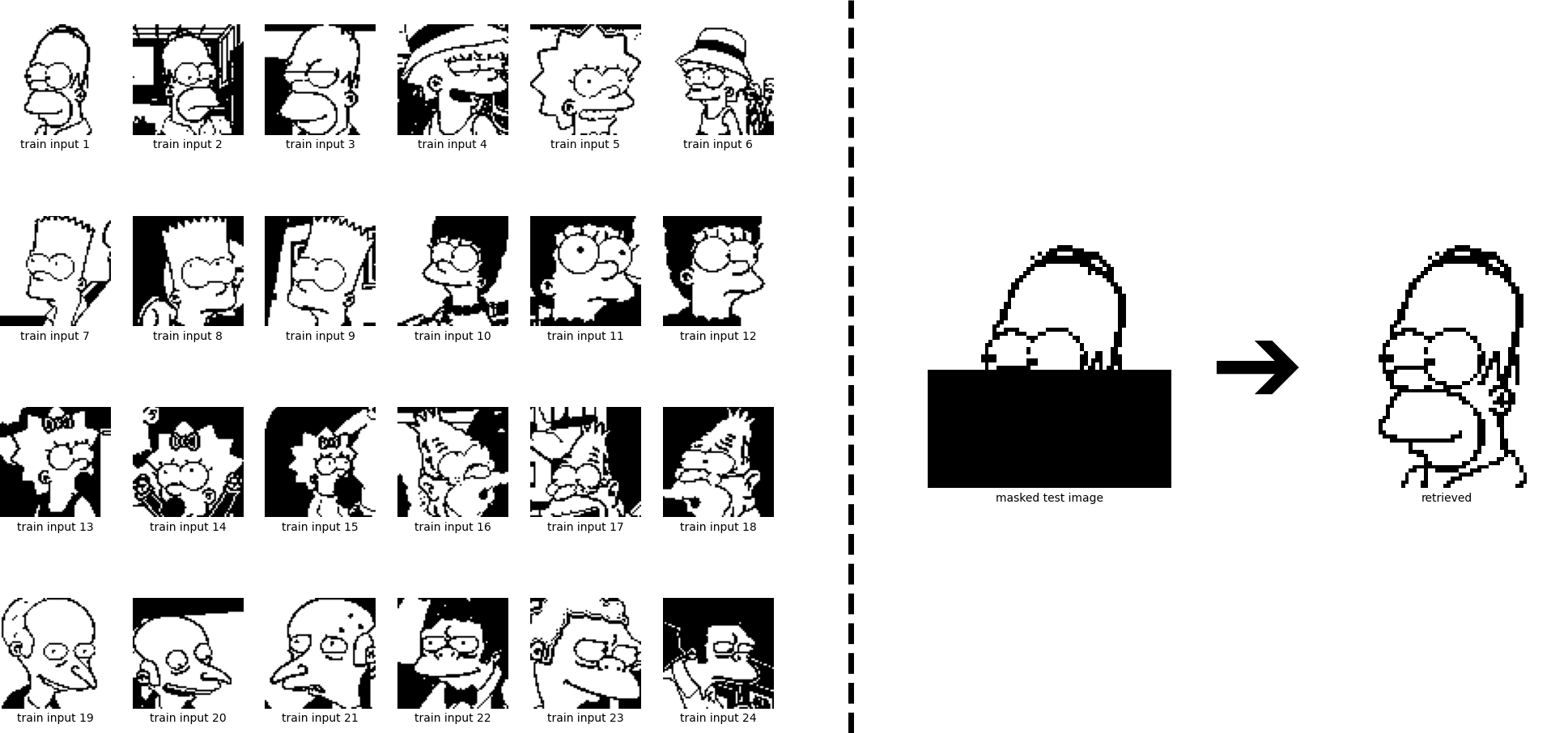
Fig. 2.70 Perfect retrieval with modern Hopfield networks. Source: https://ml-jku.github.io/hopfield-layers/
2.4. Hopfield networks is all you need (optional)
[Ramsauer et al., 2020] extend the principle to continuous patterns, i.e. vectors. Let’s put our \(P\) patterns \((\mathbf{y}^1, \mathbf{y}^2, \dots, \mathbf{y}^P)\) in a \(N \times P\) matrix:
We can define the following energy function for a vector \(\mathbf{y}\):
where:
is the log-sum-exp function and \(M\) is the maximum norm of the patterns. The first term is similar to the energy of a modern Hopfield network.
The update rule that minimizes the energy
is:

Fig. 2.71 Softmax update in a continuous Hopfield network. Source: https://ml-jku.github.io/hopfield-layers/
Why? Just read the 100 pages of mathematical proof. Take home message: these are just matrix-vector multiplications and a softmax. We can do that!
Continuous Hopfield networks can retrieve precisely continous vectors with an exponential capacity.
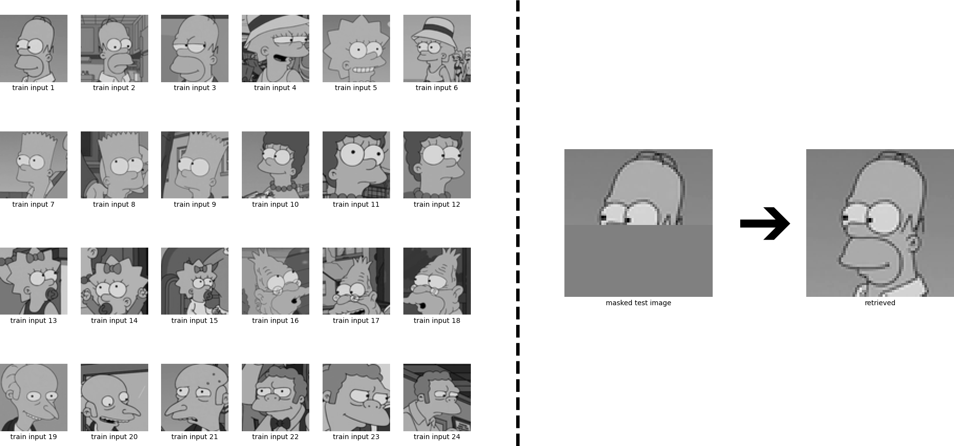
Fig. 2.72 Perfect retrieval using a continuous modern Hopfield network. Source: https://ml-jku.github.io/hopfield-layers/
The sharpness of the attractors is controlled by the temperature parameter \(\beta\). You decide whether you want single patterns or meta-stable states, i.e. combinations of similar patterns.
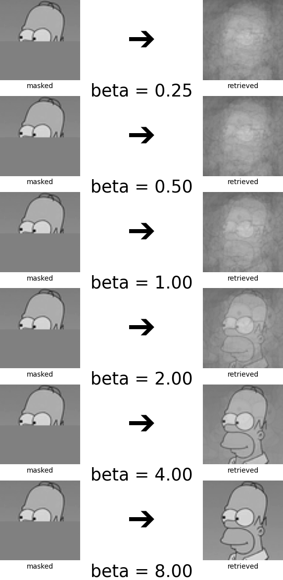
Fig. 2.73 Reconstruction with different temperatures. Source: https://ml-jku.github.io/hopfield-layers/
Why would we want that? Because it is the principle of self-attention. Which other words in the sentence are related to the current word?
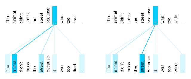
Fig. 2.74 Self-attention. Source: https://ai.googleblog.com/2017/08/transformer-novel-neural-network.html
Using the representation of a word \(\mathbf{y}\), as well as the rest of the sentence \(X\), we can retrieve a new representation \(\mathbf{y}^\text{new}\) that is a mixture of all words in the sentence.
This makes the representation of a word more context-related. The representations \(\mathbf{y}\) and \(X\) can be learned using weight matrices, so backpropagation can be used. This was the key insight of the Transformer network [Vaswani et al., 2017] that has replaced attentional RNNs in NLP.
Hopfield layers can replace the transformer self-attention with a better performance. The transformer network was introduced with the title “Attention is all you need”, hence the title of this paper… The authors claim that a Hopfield layer can also replace fully-connected layers, LSTM layers, attentional layers, but also SVM, KNN or LVQ…
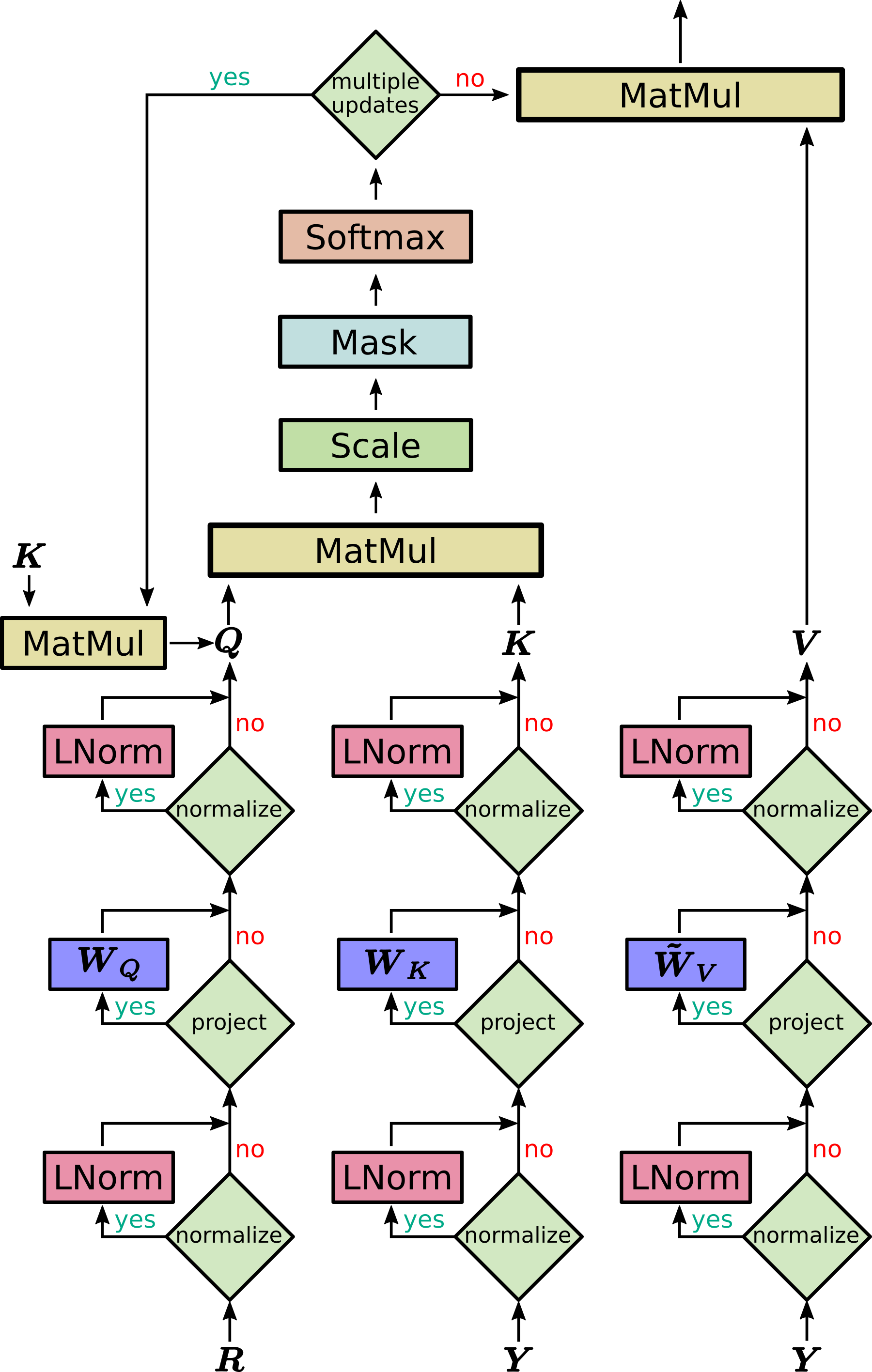
Fig. 2.75 Schematics of a Hopfield layer. Source: https://ml-jku.github.io/hopfield-layers/