3.2. Linear regression
The goal of this exercise is to implement the least mean squares algorithm (LMS) for linear regression seen in the course.
We start by importing numpy and matplotlib.
import numpy as np
import matplotlib.pyplot as plt
3.2.1. Least mean squares
To generate the data for the exercise, we will use the scikit-learn library https://scikit-learn.org. It provides a huge selection of already implemented machine learning algorithms for classification, regression or clustering.
If you use Anaconda or Colab, scikit-learn should already be installed. Otherwise, install it with pip (you may need to restart this notebook afterwards):
pip install scikit-learn
We will use the method sklearn.datasets.make_regression to generate the data. The documentation of this method is available at https://scikit-learn.org/stable/modules/generated/sklearn.datasets.make_regression.html.
The following cell imports the method:
from sklearn.datasets import make_regression
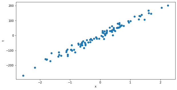
We can now generate the data. We start with the simplest case where the inputs have only one dimension. We will generate 100 samples\((x_i, t_i)\) linked by a linear relationship and some noise.
The following code generates the data:
N = 100
X, t = make_regression(n_samples=N, n_features=1, noise=15.0)
n_samples is the number of samples generates, n_features is the number of input variables and noise quantifies how the points deviate from the linear relationship.
Q: Print the shape of the arrays X and t to better understand what is generated. Visualize the dataset using matplotlib (plt.scatter). Vary the value of the noise argument in the previous cell and visualize the data again.
print(X.shape)
print(t.shape)

plt.figure(figsize=(10, 5))
plt.scatter(X, t)
plt.xlabel("x")
plt.ylabel("t")
plt.show()
(100, 1)
(100,)
Now is the time to implement the LMS algorithm with numpy.
Remember the LMS algorithm from the course:
\(w=0 \quad;\quad b=0\)
for M epochs:
\(dw=0 \quad;\quad db=0\)
for each sample \((x_i, t_i)\):
\(y_i = w \, x_i + b\)
\(dw = dw + (t_i - y_i) \, x_i\)
\(db = db + (t_i - y_i)\)
\(\Delta w = \eta \, \frac{1}{N} dw\)
\(\Delta b = \eta \, \frac{1}{N} db\)
Our linear model \(y = w \, x + b\) predicts outputs for an input \(x\). The error \(t-y\) between the prediction and the data is used to adapt the weight \(w\) and the bias \(b\) at the end of each epoch.
Q: Implement the LMS algorithm and apply it to the generated data. The Python code that you will write is almost a line-by-line translation of the pseudo-code above. You will use a learning rate eta = 0.1 at first, but you will vary this value later. Start by running a single epoch, as it will be easier to debug it, and then increase the number of epochs to 100. Print the value of the weight and bias at the end.
w = 0
b = 0

eta = 0.1

for epoch in range(100):
    dw = 0
    db = 0.0

    for i in range(N):
        # Prediction
        y = w * X[i] + b

        # LMS
        dw += (t[i] - y) * X[i]
        db += (t[i] - y)

    # Parameter updates
    w += eta * dw / N
    b += eta * db / N

print(w, b)
[95.27987845] [-1.42853731]
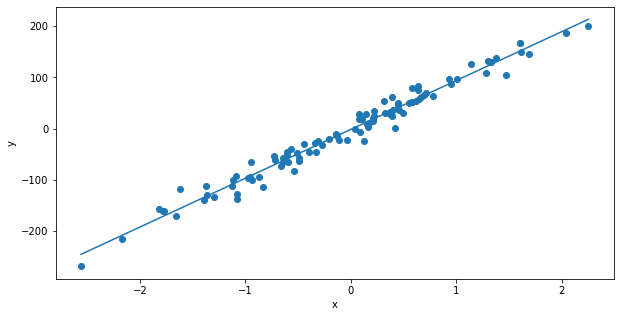
Q: Visualize the quality of the fit by superposing the learned model to the data with matplotlib.
Tip: you can get the extreme values of the xaxis with X.min() and X.max(). To visualize the model, you just need to plot a line between the points (X.min(), w*X.min()+b) and (X.max(), w*X.max()+b).
plt.figure(figsize=(10, 5))

plt.scatter(X, t)

x_axis = [X.min(), X.max()]
plt.plot(x_axis, w*x_axis + b)

plt.xlabel("x")
plt.ylabel("y")
plt.show()
Another option is to predict a value for all inputs and plot this vector \(y\) against the desired values \(t\).
Q: Make a scatter plot where \(t\) is the x-axis and \(y = w\, x + b\) is the y-axis. How should the points be arranged in the ideal case? Also plot what this ideal relationship should be.
y = w * X + b

plt.figure(figsize=(10, 5))

plt.scatter(t, y)

x_axis = [t.min(), t.max()]
plt.plot(x_axis, x_axis)

plt.xlabel("t")
plt.ylabel("y")
plt.show()
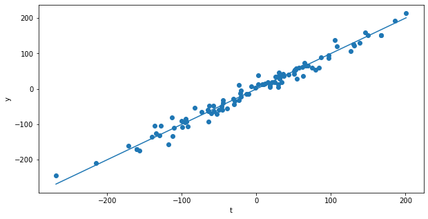
A: the points \((t, y)\) should be on a line with slope 1 and intercept 0 (i.e. t=y).
A much better method to analyse the result of the learning algorithm is to track the mean squared error (mse) after each epoch, i.e. the loss function which we actually want to minimize. The MSE is defined as:
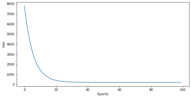
Q: Modify your LMS algorithm (either directly or copy it in the next cell) to track the mse after each epoch. After each epoch, append the mse on the training set to a list (initially empty) and plot it at the end. How does the mse evolve? Which value does it get in the end? Why? How many epochs do you actually need?
w = 0
b = 0

eta = 0.1

losses = []
for epoch in range(100):
    dw = 0
    db = 0.0
    mse = 0.0

    for i in range(N):
        # Prediction
        y = w * X[i] + b

        # LMS
        dw += (t[i] - y) * X[i]
        db += (t[i] - y)

        # mse
        mse += (t[i] - y)**2

    # Parameter updates
    w += eta*dw/N
    b += eta*db/N
    losses.append(mse/N)

print('mse:', mse/N)

plt.figure(figsize=(10, 5))
plt.plot(losses)
plt.xlabel("Epochs")
plt.ylabel("mse")
plt.show()
mse: [205.75347966]
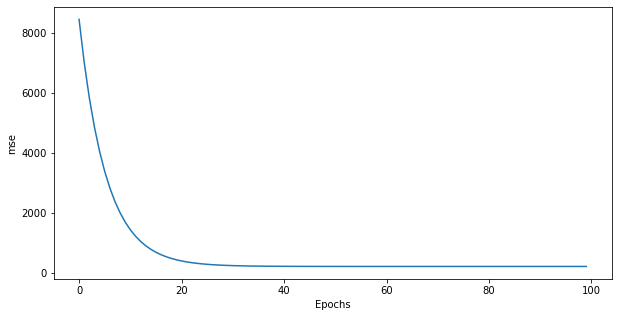
A: the mse decreases exponentially with the epochs. It never reaches 0 because of the noise in the data (try setting the noise argument in the data generator to 0 and check that the mse reaches 0). 30 or 40 epochs seem sufficient to solve the problem, nothing happens afterwards.
Let’s now study the influence of the learning rate eta=0.1 seemed to work, but is it the best value?
Q: Iterate over multiple values of eta using a logarithmic scale and plot the final mse after 100 epochs as a function of the learning rate. Conclude.
Hint: the logarithmic scale means that you will try values such as \(10^{-5}\), \(10^{-4}\), \(10^{-3}\), etc. until 1.0. In Python, you can either write explictly 0.0001 or use the notation 1e-4. For the plot, use np.log10(eta) to only display the exponent on the X-axis.
losses = []

etas = [1e-6, 1e-5, 1e-4, 1e-3, 1e-2, 1e-1, 1.0]

for eta in etas:
    w = 0
    b = 0

    for epoch in range(100):
        dw = 0
        db = 0.0
        mse = 0.0

        for i in range(N):
            # Prediction
            y = w*X[i] + b

            # LMS
            dw += (t[i] - y)*X[i]
            db += (t[i] - y)

            # mse
            mse += (t[i] - y)**2

        # Parameter updates
        w += eta*dw/N
        b += eta*db/N

    losses.append(mse/N)

print(losses)

plt.figure(figsize=(10, 5))
plt.plot(np.log10(etas), losses)
plt.xlabel("log(eta)")
plt.ylabel("mse")
plt.show()
[array([8461.50542914]), array([8448.11250949]), array([8315.36918067]), array([7099.73267265]), array([1558.81380678]), array([205.75347966]), array([205.75341538])]
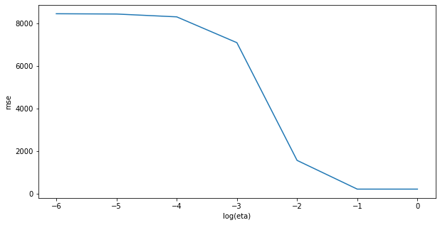
A: with small values of the learning rate, LMS does not have time to converge within 100 epochs. A learning rate of 1 is actually possible in this simple problem. Try setting eta to 2.0 and observe what happens.
3.2.2. Scikit-learn
The code that you have written is functional, but extremely slow, as you use for loops in Python. For so little data samples, it does not make a difference, but if you had millions of samples, this would start to be a problem.
The solution is to use optimized implementations of the algorithms, running in C++ or FORTRAN under the hood. We will use here the LMS algorithm provided by scikit-learn as you have already installed it and it is very simple to use. Note that one could use tensorflow too, but that would be killing a fly with a sledgehammer.
scikit-learn provides a LinearRegression object that implements LMS. The documentation is at: https://scikit-learn.org/stable/modules/generated/sklearn.linear_model.LinearRegression.html.
You simply import it with:
from sklearn.linear_model import LinearRegression
You create the object with:
reg = LinearRegression()
reg is now an object with different methods (fit(), predict()) that accept any kind of data and performs linear regression.
To train the model on the data \((X, t)\), simply use:
reg.fit(X, t)
The parameters of the model are obtained with reg.coef_ for \(w\) and reg.intercept_ for \(b\).
You can predict outputs for new inputs using:
y = reg.predict(X)
Q: Apply linear regression on the data using scikit-learn. Check the model parameters after learning and compare them to what you obtained previously. Print the mse and make a plot comparing the predictions with the data.
from sklearn.linear_model import LinearRegression

# Linear regression
reg = LinearRegression()
reg.fit(X, t)

print(reg.coef_, reg.intercept_)

# Prediction
y = reg.predict(X)

# mse
mse = np.mean((t - y)**2)
print('mse:', mse)

plt.figure(figsize=(10, 5))
plt.scatter(t, y)
x_axis = [t.min(), t.max()]
plt.plot(x_axis, x_axis)
plt.xlabel("t")
plt.ylabel("y")
plt.show()
[95.28734628] -1.426580793575432
mse: 205.75341537754272

A: No need to select the right learning rate, fast and error-free.
3.2.3. Delta learning rule
Let’s now implement the online version of LMS, the delta learning rule. The only difference is that the parameter updates are applied immediately after each example is evaluated, not at the end of training.
\(w=0 \quad;\quad b=0\)
for M epochs:
for each sample \((x_i, t_i)\):
\(y_i = w \, x_i + b\)
\(\Delta w = \eta \, (t_i - y_i ) \, x_i\)
\(\Delta b = \eta \, (t_i - y_i)\)
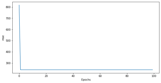
Q: Implement the delta learning rule for the regression problem with eta = 0.1. Plot the evolution of the mse and compare it to LMS.
w = 0
b = 0

eta = 0.1

losses = []
for epoch in range(100):

    mse = 0.0

    for i in range(N):
        # Prediction
        y = w * X[i] + b

        # Delta learning rule
        w += eta * (t[i] - y) * X[i]
        b += eta * (t[i] - y)

        # mse
        mse += (t[i] - y)**2

    losses.append(mse/N)

print('mse:', mse/N)

plt.figure(figsize=(10, 5))
plt.plot(losses)
plt.xlabel("Epochs")
plt.ylabel("mse")
plt.show()
mse: [241.05201205]
y = w * X + b

plt.figure(figsize=(10, 5))

plt.scatter(t, y)

x_axis = [t.min(), t.max()]
plt.plot(x_axis, x_axis)

plt.xlabel("t")
plt.ylabel("y")
plt.show()

A: The delta learning rule converges faster, but the final mse is higher. This is due to the learning rate as shown in the next question.
Q: Vary the learning rate logarithmically as for LMS and conclude.
losses = []

etas = [1e-6, 1e-5, 1e-4, 1e-3, 1e-2, 1e-1]

for eta in etas:

    w = 0
    b = 0

    for epoch in range(100):

        mse = 0.0

        for i in range(N):
            # Prediction
            y = w * X[i] + b

            # Delta learning rule
            w += eta * (t[i] - y) * X[i]
            b += eta * (t[i] - y)

            # mse
            mse += (t[i] - y)**2

    losses.append(mse/N)

print(losses)

plt.figure(figsize=(10, 5))
plt.plot(np.log10(etas), losses)
plt.xlabel("eta")
plt.ylabel("mse")
plt.show()
[array([8314.66609921]), array([7094.25080431]), array([1557.7207601]), array([206.18470859]), array([209.94231293]), array([241.05201205])]
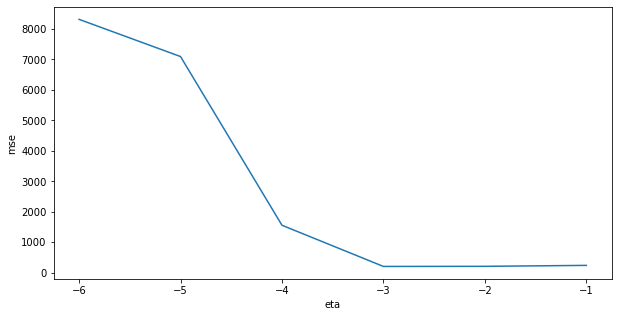
A: The optimal value of eta is now 0.001, higher learning rates lead to worse mse. One explanation is that the true learning rate of LMS is eta/N = 0.001, not eta=0.1. When using 0.001 for the learning, the delta learning rule behaves exactly like LMS:
w = 0
b = 0

eta = 0.001

losses = []
for epoch in range(100):

    mse = 0.0

    for i in range(N):
        # Prediction
        y = w * X[i] + b

        # Delta learning rule
        w += eta * (t[i] - y) * X[i]
        b += eta * (t[i] - y)

        # mse
        mse += (t[i] - y)**2

    losses.append(mse/N)

print('mse:', mse/N)

plt.figure(figsize=(10, 5))
plt.plot(losses)
plt.xlabel("Epochs")
plt.ylabel("mse")
plt.show()
mse: [206.18470859]
