.md .pdf

Contents

4. Unsupervised Hebbian learning

Guest lecturer: Dr. Michael Teichmann.

Slides: pdf

4.1. What is Hebbian learning?

Donald Hebb postulates 1949 in its book The Organization of Behavior how long lasting cellular changes are induced in the nervous system:

When an axon of cell A is near enough to excite a cell B and repeatedly or persistently takes part in firing it, some growth process or metabolic change takes place in one or both cells such that A’s efficiency, as one of the cells firing B, is increased.

which is often simplified to:

Neurons wire together if they fire together.

Based on this principle, a basic computational rule can be formulated, where the weight change is proportional to the product of activation values:

\[ \Delta w_{ij} = \eta \, r_i \, r_j \]

where \(r_i\) is the pre-synaptic activity of neuron \(i\), \(r_j\) the post-synaptic activity of neuron \(j\) and \(w_{ij}\) the weight from neuron \(i\) to \(j\).

Fig. 4.31 Two connected neurons.

Hebbian learning requires no other information than the activities, such as labels or error signals: it is an unsupervised learning method. Hebbian learning is not a concrete learning rule, it is a postulate on the fundamental principle of biological learning. Because of its unsupervised nature, it will rather learn frequent properties of the input statistics than task-specific properties. It is also called a correlation-based learning rule.

A useful Hebbian-based learning rule has to respect several criteria [Gerstner & Kistler, 2002]:

1. Locality: The weight change should only depend on the activity of the two neurons and the synaptic weight itself. \(\Delta w_{ij} = F(w_{ij}; r_i; r_j)\)

2. Cooperativity: Hebb’s postulate says cell A “takes part in firing it”, which implicates that both neurons must be active to induce a weight increase.

3. Synaptic depression: whilw Hebb’s postulate refers only to conditions to strengthen the synapses, a mechanism for decreasing weights is necessary for any useful learning rule.

4. Boundedness: To be realistic, weights should remain bounded in a certain range. The dependence of the learning on \(w_{ij}\) or \(r_j\) can be used for bounding the weights.

5. Competition: The weights grow at the expense of other weights. This can be implemented by a local form of weight vector normalization.

6. Long-term stability: For adaptive systems, care must be taken that previously learned information is not lost. This is called the “stability-plasticity dilemma”.

4.2. Implementations of Hebbian learning rules

4.2.1. Simple Hebbian learning rule

In the most basic formulation, learning depends only on the presynaptic \(r_i\) and postsynaptic \(r_j\) firing rates and a learning rate \(\eta\) (correlation-based learning principle):

\[ \Delta w_{ij} = \eta \, r_i \, r_j \]

If the postsynaptic activity is computed over multiple input synapses:

\[\begin{split} r_j = \sum_i w_{ij} \, r_i = \mathbf{r}^T \times \mathbf{w}_j \\ \end{split}\]

then the learning rule accumulates the auto-correlation matrix \(Q\) of the input vector \(\mathbf{r}\):

\[ \Delta \mathbf{w}_j = \eta \, \mathbf{r} \, r_j = \eta \, \mathbf{r} \times \mathbf{r}^T \times \mathbf{w}_j = \eta \, Q \times \mathbf{w}_j \]

When multiple input vectors are presented, \(Q\) represents the correlation matrix of the inputs:

\[ Q = \mathbb{E}_{\mathbf{r}} [\mathbf{r} \times \mathbf{r}^T] \]

Thus, Hebbian plasticity is assigning strong weights to frequently co-occurring input elements.

4.2.2. Covariance-based Hebbian learning

The covariance between two random variables \(X\) and \(Y\) is defined by:

\[\begin{split}\begin{aligned} \text{cov}(X,Y) &= \mathbb{E}(X- \mathbb{E}(X)) \, \mathbb{E}(Y-\mathbb{E}(Y))\\ &\\ &= \mathbb{E}(XY)- \mathbb{E}(X) \, \mathbb{E}(Y) \\ \end{aligned}\end{split}\]

One property of the covariance is that it is zero for independent variables and positive for dependent variables. However, it just measures linear independence and ignores higher order dependencies. It is useful to learn meaningful weights only between statistically dependent neurons.

With the following formulation, the weight change is relative to the covariance of the activity of the connected neurons:

\[\begin{split}\begin{aligned} \Delta w_{ij} &= \eta \, (r_i-\theta_i) \, (r_j-\theta_j)\\ \end{aligned}\end{split}\]

where \(\theta_i\) and \(\theta_j\) are estimates of the expectation of the pre- and post-synaptic activities, for example through a moving average:

\[\begin{split}\begin{aligned} \theta_i & = \alpha \, \theta_i + (1 - \alpha) \, r_i \\ &\\ \theta_j & = \beta \, \theta_j + (1 - \beta) \, r_j \\ \end{aligned}\end{split}\]

Note that with covariance-based learning, weight can both increase (LTP) and decrease (LTD). Some variants of covariance-based Hebbian only use a threshold on one of the terms:

\[\begin{split}\begin{aligned} \Delta w_{ij} &= \eta \, r_i \, (r_j-\theta) = \eta \, (r_i \, r_j - \theta \, r_i)\\ &\\ \Delta w_{ij} &= \eta \, (r_i-\theta) \, r_j = \eta \, (r_i \, r_j- \theta \, r_j) \end{aligned}\end{split}\]

The previous implementations lack any bound for the weight increase. Since the correlation of input and output increases through learning the weight would grow without limits. In the case of anti-correlated neurons, the weights could also become negative for covariance-based learning.

There are several ways to bound the weights:

• Hard bounds

\[ w_{min}\le w_{ij} \le w_{max} \]

• Soft bounds

\[ \Delta w_{ij} = \eta \, r_i \, r_j \, (w_{ij} - w_{min}) \, (w_{max}-w_{ij}) \]

• Normalized weight vector length [Oja, 1982]:

\[ \Delta w_{ij} = \eta \, (r_i \, r_j - \alpha \, r_j^2 \, w_{ij}) \]

• Rate-based threshold adaption [Bienenstock et al., 1982].

4.2.3. Oja learning rule

Erkki Oja [Oja, 1982] found a formulation which normalizes the length of a weight vector by a local operation, fulfilling the first criterium for Hebbian learning.

\[ \Delta w_{ij} = \eta \, (r_i \, r_j - \alpha \, r_j^2 \, w_{ij}) \]

\(\alpha \, r_j^2 \, w_{ij}\) is a regularization term: when the weight \(w_{ij}\) or the postsynaptic activity \(r_j\) are too high, the term cancels the “Hebbian” part \(r_i \, r_j\) and decreases the weight.

Oja has shown that with this equation the norm of the weight vector converges to a constant value determined by the parameter \(\alpha\):

\[ ||\mathbf{w}||^2 = \frac{1}{\alpha} \]

To come to the solution the relation between input and output \(r_j = \mathbf{r} \times \mathbf{w}^T\) and a Taylor expansion over \(\mathbf{w}\) has been used.

4.2.4. Bienenstock-Cooper-Monroe (BCM) learning rule

In the Bienenstock-Cooper-Monroe (BCM) learning rule [Bienenstock et al., 1982] [Intrator & Cooper, 1992], the threshold \(\theta\) averages the square of the post-synaptic activity, i.e. its second moment (\(\approx\) variance).

\[\begin{split}\begin{aligned} \Delta w_{ij} &= \eta \, r_i \, (r_j - \theta) \, r_j \, f'(net)\\ &\\ \theta &= \mathbb{E} [r_j^2] \\ \end{aligned}\end{split}\]

When the short-term trace \(\theta\) over the past activities of \(r_j\) increases, the fraction of events leading to synaptic depression increases.

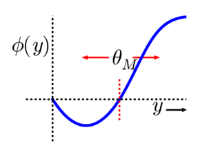
Fig. 4.32 BCM learning rule [Bienenstock et al., 1982]. Source: http://www.scholarpedia.org/article/BCM_theory.

4.2.5. Spike-Time-Dependent Plasticity (STDP)

The brain transmits neuronal activity majorly via generation of short electrical impulses, called spikes. The timing of these spikes might convey additional information over the firing rate, which we regarded before. Spike-based neural networks are also a technical way to transmit information with a very high energy efficiency (neuromorphic hardware). An important aspect of STDP is the temporal asymmetric learning window. A spike that arrives slightly before the postsynaptic spike is likely to cause this one. Thus, STDP learning rules can incorporate temporal aspects implying causality, an important implicit aspect of the cooperativity property of Hebbian learning.

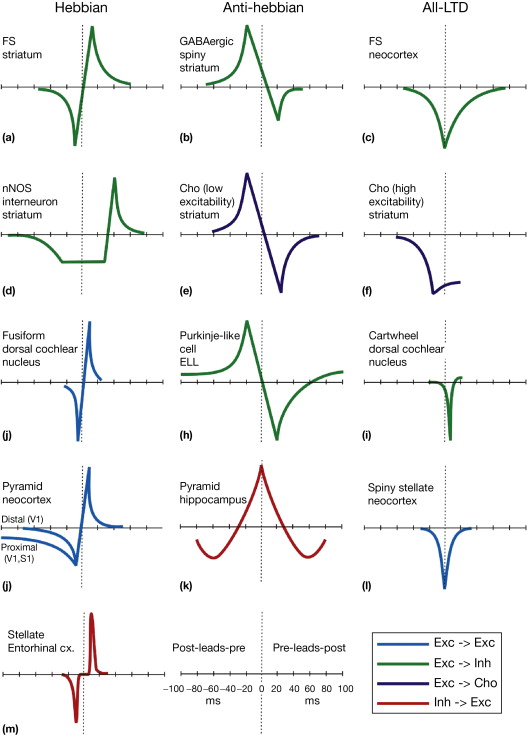
Fig. 4.33 STDP learning rule. Source: https://doi.org/10.1016/C2011-0-07732-3

4.3. Hebbian Neural Networks

4.3.1. Perceptron

What does a layer of multiple neurons learn with Hebbian learning? Erkki Oja (1982) has shown that his learning rule converges for linear neurons to the first principle component of the input data. A principle component is an eigenvector of the covariance matrix of the input data. The first principle component is the eigenvector with the largest variance, having the highest eigenvalue. A network of these neurons appears not very useful, as all neurons will just learn the first principle component. An additional element is required providing differentiation between the neurons.

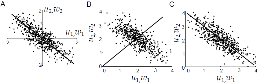
Fig. 4.34 Principle components. Source: [Dayan & Abbott, 2001].

There are several methods existing differentiating the neuron responses, e.g.:

1. Winner-take-all competition

   • Only the neuron with the highest response is selected for learning.

   • In practice k-winner-take-all is often used, letting the k strongest neurons learn.

2. A recurrent circuit providing a competitive signal.

   • The neurons compete with their neighbors to become active to learn.

   • In the brain this is not done directly, it is done via a special neuron type, called inhibitory neurons.

   • Inhibitory neurons form only synapses reducing the activity of the postsynaptic neuron (Dale’s law).

   • Inhibition can be implemented in different manners.

4.3.2. Inhibition

Modulatory inhibition divides the excitation of the postsynaptic neuron by the received inhibition coming from the neighboring units. Scaling the neuronal gain and non-linearly separating the activity values of the neurons in the way that high activities remain high, but lower activities are suppressed.

\[ r_j(\sigma,E,I)=\frac{E}{\sigma+E+I} \]

with excitation E, inhibition I, and \(\sigma\) scaling the strength of the normalization.

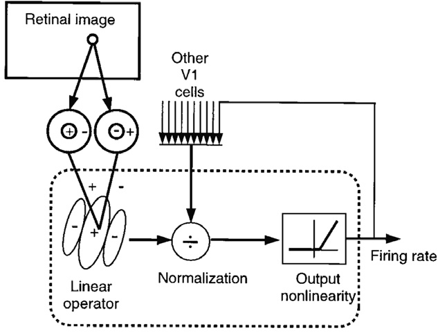
Fig. 4.35 Models of normalization as feedback circuit for V1 cells. Source: Graham, N. V. (2011). Beyond multiple pattern analyzers modeled as linear filters (as classical V1 simple cells): useful additions of the last 25 years. Vision Research, 51(13), 1397–1430. https://doi.org/10.1016/j.visres.2011.02.007

Subtractive inhibition means that the inhibitory currents are subtracted from the excitatory one. In a recurrent circuit highly active neurons reduce the activity of their neighboring neurons and limit their ability to inhibit other neurons. This is called shunting inhibition.

\[ r_j(E,I)=E-I \]

Depending how the weights are arranged this can implement a continuum from winner-take-all competition (equal and strong weights) to very specific competition between particular neurons (e.g. penalizing similar neurons).

A method to learn weights providing a penalty for similarly active neurons is anti-Hebbian learning. Hebbian learning can easily turned into anti-Hebbian learning by switching the sign of the weight change or switching the effect of the weight from excitatory to inhibitory. Covariance-based weight change [Vogels et al., 2011]:

\[ \Delta c_{ij} = r_i \, r_j - r_i \, \rho_0 \]

Weight relative to covariance:

\[ \Delta c_{ij} = r_i \, r_j - r_i \, \rho_0 \, (1 + c_{ij}) \]

The equilibrium point of the equation is reached, when the weight indicates by which factor the product of the expectation values \(r_i \rho_0\) has to be multiplied to be equal to the expectation value of the product of the activities \(r_i r_j\).

From a theoretical viewpoint anti-Hebbian learned competition aims to minimize linear dependencies between the activities. When having independent neural activities than the information encoded by a population of neurons is maximal [Simoncelli & Olshausen, 2001].

What about the boundedness issue? Oja normalization is based on the fact that the postsynaptic activity is caused by the presynaptic activity and the weight strength. This is only true for excitatory weights. Inhibitory weights reduce the activity. This causes a softbound effect:

• When the inhibitory weight increases, the activity decreases.

• With lower activities the weight change gets slower, until it stops when the neuron remains inactive.

Formulations where the weight is relative to the covariance additionally saturate at their equilibrium point.

4.4. Information representation (optional)

Since Hebbian and anti-Hebbian learning are restricted to use only local information, there is no global objective what a population of these neurons should represent. Competition between the neurons induce differences in their response patterns, but might not control that all neurons convey information. There are two issues:

• A single pattern can get dominant because of differences in the activity.

\[ E(w_{ij}) = E(r_i \, r_j) - E(r_i) \, E(r_j) \]

If the activity of a particular input neuron \(r_i\) is by average higher than the activity of other input neurons, then its weight value gets higher than the weight of a similarly correlated but less active neuron. This effect is strengthen over multiple layers, causing a dominance of a few patterns. Thus, the activities have to be balanced to avoid an imbalanced input to the next layer.

• Neurons can become permanently inactive or unresponsive to changing input.

This can be avoided by aiming for a similar operating point of the neurons, by keeping:

• All neurons active, to use the full capacity of the neuronal population.

• All neurons in a similar range, so that no neuron can dominate the learnings of subsequent layers.

4.4.1. Homeostasis

In Hebbian learning, the amount of weight decrease and increase can be regulated to achieve a certain activity range. [Clopath et al., 2010] regulate the strength of the weight decrease \(A_{LTD}\) by relating the average membrane potential \(\bar{\bar u}\) to a reference value \(u_{ref}^2\), defining a target activity with that:

\[ A_{LTD}(\bar{\bar u})=A_{LTD} \, \frac{\bar{\bar u}^2}{u_{ref}^2} \]

BCM learning adapts the threshold based on the average activity of the neuron, facilitating or impeding weight increases and decreases:

\[ \Delta w_{ij} = \eta \, r_i \, (r_j - \theta) \, r_j \, f'(net) \]

\[ \theta = \mathbb{E} [r_j^2] \]

In anti-Hebbian learning, the amount of inhibition a neuron receives is up or downregulated to achieve a certain average activity. [Vogels et al., 2011] define a target activity of the postsynaptic neuron \(\rho_0\), the amount of inhibition is up or downregulated to reach this activity:

\[ \Delta w_{ij} = r_i \, (r_j - \rho_0) \]

4.4.2. Intrinsic plasticity

First option: forcing a certain activity distribution, through adapting the activation function.

[Joshi & Triesch, 2009] adapt the parameters of the transfer function \(g(u)\), by minimizing the Kullback-Leibler divergence between the neuron’s activity and an exponential distribution. The update rules for the parameters \(r_0, u_0, u_\alpha\) have been derived via stochastic gradient descent:

\[ g(u) = r_0 \, \log \left( 1 + e^\frac{u-u_0}{u_\alpha} \right) \]

\[ \Delta r_0 = \frac{\eta}{r_0} \left( 1- \frac{g}{\mu} \right) \]

\[ \Delta u_0 = \frac{\eta}{u_\alpha} \left( \left( 1+\frac{r_0}{\mu} \right) \left( 1-e^\frac{-g}{r_0} \right) -1 \right) \]

\[ \Delta u_\alpha = \frac{\eta}{u_\alpha} \left( \frac{u-u_0}{u_\alpha} \left( \left( 1+\frac{r_0}{\mu} \right) \left( 1-e^\frac{-g}{r_0} \right) -1 \right) -1 \right) \]

Second option: regulating the first moments of activity (mean, variance) and by adapting the activation function.

Teichmann and Hamker (2015) adapt the parameters of a rectified linear transfer function, by regulating the threshold \(\theta_j\) and slope \(a_j\), to achieve a similar mean and variance of all neurons within a layer:

\[ \Delta r_j = a_j \left( \sum_i w_{ij} \, r_i - \sum_{k, k \ne j} c_{kj} \, r_k - \theta_j \right) -r_j \]

\[ \Delta \theta_j = (r_j - \theta_{target}) \]

\[ \Delta a_j = (a_{target} -r_j^2) \]

Source: Teichmann, M. and Hamker, F. H. (2015). Intrinsic Plasticity: A Simple Mechanism to Stabilize Hebbian Learning in Multilayer Neural Networks. In T. Villmann & F.-M. Schleif (Eds.), Machine Learning Reports 03/2015 (pp. 103–111) https://www.techfak.uni-bielefeld.de/~fschleif/mlr/mlr_03_2015.pdf

4.4.3. Supervised Hebbian learning

Large parts of the plasticity in the brain is thought to be Hebbian, this means it uses local information and learns unsupervised. However the brain also is largely recurrent, information flows in all directions and this information could guide neighboring or preceding processing stages. If such an information influences the activity of a neuron then it also influences the learning on the other synapses of this neuron.

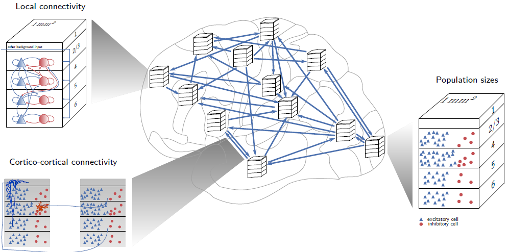
Fig. 4.36 Recurrent connectivity in the visual cortex. Source: Schmidt, M., Diesmann, M. and Albada, S. J. Van. (2018). Multi-scale account of the network structure of macaque visual cortex. Brain Structure and Function, 223(3), 1409–1435. https://doi.org/10.1007/s00429-017-1554-4

In supervised Hebbian learning the postsynaptic activity is fully controlled. With that the subset of inputs which should evoke activity can be selected.

\[ \Delta w_{ij} = r_i \, t - \alpha \, w_{ij} \]

The supervised Hebbian learning principle can be extended to a form of top-down learning. A top-down signal, conveying additional modulatory information, modulates or contributes partially to the neuronal activity.

We can illustrate the effect by splitting the plasticity term into bottom-up and the top-down parts.

\[ r'_j= \gamma \, r_j + (1-\gamma) \, t \]

\[ \Delta w_{ij} = r_i \, r'_j- \alpha \, {r'_j}^2 \, w_{ij} \]

Depending on \(\gamma\), the top-down signal contributes to the activity, it implements a continuum between unsupervised and supervised Hebbian learning. The weight change does not depend on the actual performance, therefore error correcting learning rules are required.

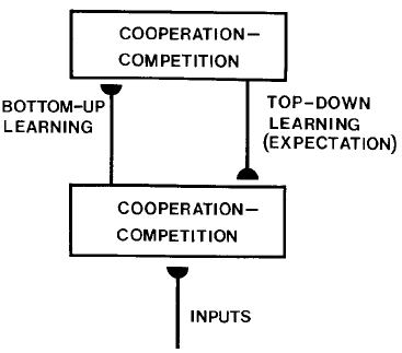
Fig. 4.37 Source: Grossberg, S. (1988). Nonlinear neural networks: Principles, mechanisms, and architectures. Neural Networks, 1(1), 17–61. https://doi.org/10.1016/0893-6080(88)90021-4

4.5. Summary

• Hebbian learning postulates properties of biological learning.

• There is no concrete implementation of Hebbian learning. Algorithms have to fulfill the properties: locality, cooperativity, synaptic depression, boundedness, competition, and long term stability.

• Hebbian learning exploits the statistics of its input and learns frequent patterns. Like the first principle component.

• Beside differences from random initialization of the weights, all neurons would learn the same pattern, when having the same inputs. Thus, Hebbian learning requires a mechanism for competition for differentiation.

• Recurrent inhibitory connections induce competition by penalizing similar activities of the neurons. With that dependencies are reduced and the neural code gets efficient in terms of the information it conveys.

• However, imbalances in the activity can harm Hebbian learning in subsequent layers. Or inactive neurons reduce the information. Thus, the operating point of the neurons has to be adjusted.

• The operating point can be modified by set points in the Hebbian or anti-Hebbian learning rules. Or by regulating the transfer function of the neurons to achieve either a particular activity distribution or similar response properties like mean and variance.

• Hebbian learning can be extended by top-down signals and implement a continuum between supervised and unsupervised learning. This might help to reduce the dependency on large amounts of labeled data of supervised learning algorithms.

previous

3. Reservoir computing

next

5. Spiking neural networks