.md .pdf

Contents

4. Linear classification

Slides: pdf

4.1. Hard linear classification

The training data \(\mathcal{D}\) is composed of \(N\) examples \((\mathbf{x}_i, t_i)_{i=1..N}\) , with a d-dimensional input vector \(\mathbf{x}_i \in \Re^d\) and a binary output \(t_i \in \{-1, +1\}\). The data points where \(t = + 1\) are called the positive class, the other the negative class.

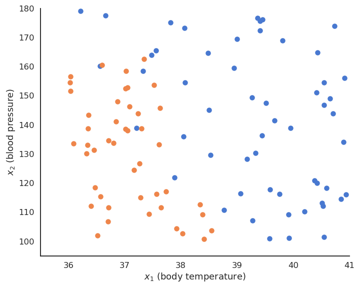
Fig. 4.1 Binary linear classification of 2D data.

For example, the inputs \(\mathbf{x}_i\) can be images (one dimension per pixel) and the positive class corresponds to cats (\(t_i = +1\)), the negative class to dogs (\(t_i = -1\)).

Fig. 4.2 Binary linear classification of cats vs. dogs images. Source: http://adilmoujahid.com/posts/2016/06/introduction-deep-learning-python-caffe

We want to find the hyperplane \((\mathbf{w}, b)\) of \(\Re^d\) that correctly separates the two classes.

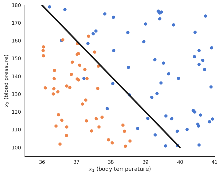
Fig. 4.3 The hyperplane separates the input space into two regions.

For a point \(\mathbf{x} \in \mathcal{D}\), \(\langle \mathbf{w} \cdot \mathbf{x} \rangle +b\) is the projection of \(\mathbf{x}\) onto the hyperplane \((\mathbf{w}, b)\).

• If \(\langle \mathbf{w} \cdot \mathbf{x} \rangle +b > 0\), the point is above the hyperplane.

• If \(\langle \mathbf{w} \cdot \mathbf{x} \rangle +b < 0\), the point is below the hyperplane.

• If \(\langle \mathbf{w} \cdot \mathbf{x} \rangle +b = 0\), the point is on the hyperplane.

Fig. 4.4 Projection on an hyperplane.

By looking at the sign of \(\langle \mathbf{w} \cdot \mathbf{x} \rangle +b\), we can predict the class.

\[\begin{split}\text{sign}(x) = \begin{cases} +1 \; \text{if} \; x \geq 0 \\ -1 \; \text{if} \; x < 0 \\ \end{cases}\end{split}\]

Binary linear classification can therefore be made by a single artificial neuron using the sign transfer function.

\[ y = f_{\mathbf{w}, b} (\mathbf{x}) = \text{sign} ( \langle \mathbf{w} \cdot \mathbf{x} \rangle +b ) = \text{sign} ( \sum_{j=1}^d w_j \, x_j +b ) \]

\(\mathbf{w}\) is the weight vector and \(b\) is the bias.

Linear classification is the process of finding an hyperplane \((\mathbf{w}, b)\) that correctly separates the two classes. If such an hyperplane can be found, the training set is said linearly separable. Otherwise, the problem is non-linearly separable and other methods have to be applied (MLP, SVM…).

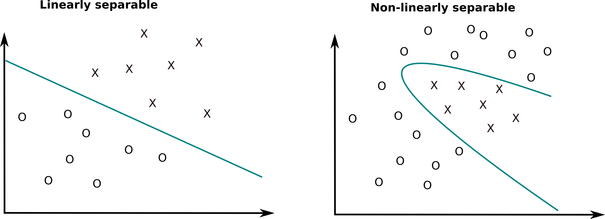
Fig. 4.5 Linearly and non-linearly spearable datasets.

4.1.1. Perceptron algorithm

The Perceptron algorithm tries to find the weights and biases minimizing the mean square error (mse) or quadratic loss:

\[\mathcal{L}(\mathbf{w}, b) = \mathbb{E}_\mathcal{D} [(t_i - y_i)^2] \approx \frac{1}{N} \, \sum_{i=1}^{N} (t_i - y_i)^2\]

When the prediction \(y_i\) is the same as the data \(t_i\) for all examples in the training set (perfect classification), the mse is minimal and equal to 0. We can apply gradient descent to find this minimum.

\[ \Delta \mathbf{w} = - \eta \, \nabla_\mathbf{w} \, \mathcal{L}(\mathbf{w}, b) \]

\[ \Delta b = - \eta \, \nabla_b \, \mathcal{L}(\mathbf{w}, b) \]

Let’s search for the partial derivative of the quadratic error function with respect to the weight vector:

\[ \nabla_\mathbf{w} \, \mathcal{L}(\mathbf{w}, b) = \nabla_\mathbf{w} \, \frac{1}{N} \, \sum_{i=1}^{N} (t_i - y_i )^2 = \frac{1}{N} \, \sum_{i=1}^{N} \nabla_\mathbf{w} \, (t_i - y_i )^2 = \frac{1}{N} \, \sum_{i=1}^{N} \nabla_\mathbf{w} \, \mathcal{l}_i (\mathbf{w}, b) \]

Everything is similar to linear regression until we get:

\[ \nabla_\mathbf{w} \, \mathcal{l}_i (\mathbf{w}, b) = - 2 \, (t_i - y_i) \, \nabla_\mathbf{w} \, \text{sign}( \langle \mathbf{w} \cdot \mathbf{x}_i \rangle +b) \]

In order to continue with the chain rule, we would need to differentiate \(\text{sign}(x)\).

\[ \nabla_\mathbf{w} \, \mathcal{l}_i (\mathbf{w}, b) = - 2 \, (t_i - y_i) \, \text{sign}'( \langle \mathbf{w} \cdot \mathbf{x}_i \rangle +b) \, \mathbf{x}_i \]

But the sign function is not differentiable… We will simply pretend that the sign() function is linear, with a derivative of 1:

\[ \nabla_\mathbf{w} \, \mathcal{l}_i (\mathbf{w}, b) = - 2 \, (t_i - y_i) \, \mathbf{x}_i \]

The update rule for the weight vector \(\mathbf{w}\) and the bias \(b\) is therefore the same as in linear regression:

\[ \Delta \mathbf{w} = \eta \, \frac{1}{N} \, \sum_{i=1}^{N} (t_i - y_i) \, \mathbf{x}_i \]

\[ \Delta b = \eta \, \frac{1}{N} \, \sum_{i=1}^{N} (t_i - y_i ) \]

By applying gradient descent on the quadratic error function, one obtains the following algorithm:

Batch perceptron

• for \(M\) epochs:

  • \(\mathbf{dw} = 0 \qquad db = 0\)

  • for each sample \((\mathbf{x}_i, t_i)\):

    • \(y_i = \text{sign}( \langle \mathbf{w} \cdot \mathbf{x}_i \rangle + b)\)

    • \(\mathbf{dw} = \mathbf{dw} + (t_i - y_i) \, \mathbf{x}_i\)

    • \(db = db + (t_i - y_i)\)

  • \(\Delta \mathbf{w} = \eta \, \frac{1}{N} \, \mathbf{dw}\)

  • \(\Delta b = \eta \, \frac{1}{N} \, db\)

This is called the batch version of the Perceptron algorithm. If the data is linearly separable and \(\eta\) is well chosen, it converges to the minimum of the mean square error.

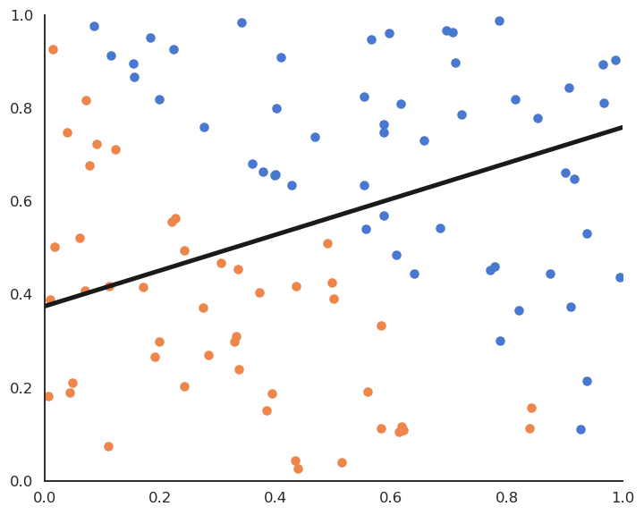
Fig. 4.6 Batch perceptron algorithm.

The Perceptron algorithm was invented by the psychologist Frank Rosenblatt in 1958. It was the first algorithmic neural network able to learn linear classification.

Online perceptron algorithm

• for \(M\) epochs:

  • for each sample \((\mathbf{x}_i, t_i)\):

    • \(y_i = \text{sign}( \langle \mathbf{w} \cdot \mathbf{x}_i \rangle + b)\)

    • \(\Delta \mathbf{w} = \eta \, (t_i - y_i) \, \mathbf{x}_i\)

    • \(\Delta b = \eta \, (t_i - y_i)\)

This algorithm iterates over all examples of the training set and applies the delta learning rule to each of them immediately, not at the end on the whole training set. One could check whether there are still classification errors on the training set at the end of each epoch and stop the algorithm. The delta learning rule depends as always on the learning rate \(\eta\), the error made by the prediction (\(t_i - y_i\)) and the input \(\mathbf{x}_i\).

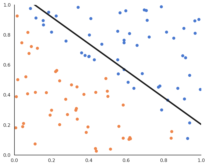
Fig. 4.7 Online perceptron algorithm.

4.1.2. Stochastic Gradient descent

The mean square error is defined as the expectation over the data:

\[\mathcal{L}(\mathbf{w}, b) = \mathbb{E}_\mathcal{D} [(t_i - y_i)^2]\]

Batch learning uses the whole training set as samples to estimate the mse:

\[\mathcal{L}(\mathbf{w}, b) \approx \frac{1}{N} \, \sum_{i=1}^{N} (t_i - y_i)^2\]

\[ \Delta \mathbf{w} = \eta \, \frac{1}{N} \sum_{i=1}^{N} (t_i - y_i ) \, \mathbf{x_i} \]

Online learning uses a single sample to estimate the mse:

\[\mathcal{L}(\mathbf{w}, b) \approx (t_i - y_i)^2\]

\[ \Delta \mathbf{w} = \eta \, (t_i - y_i) \, \mathbf{x_i} \]

Batch learning has less bias (central limit theorem) and is less sensible to noise in the data, but is very slow. Online learning converges faster, but can be instable and overfits (high variance).

In practice, we use a trade-off between batch and online learning called Stochastic Gradient Descent (SGD) or Minibatch Gradient Descent.

The training set is randomly split at each epoch into small chunks of data (a minibatch, usually 32 or 64 examples) and the batch learning rule is applied on each chunk.

\[ \Delta \mathbf{w} = \eta \, \frac{1}{K} \sum_{i=1}^{K} (t_i - y_i) \, \mathbf{x_i} \]

If the batch size is well chosen, SGD is as stable as batch learning and as fast as online learning. The minibatches are randomly selected at each epoch (i.i.d).

Note

Online learning is a stochastic gradient descent with a batch size of 1.

4.2. Maximum Likelihood Estimation

Let’s consider \(N\) samples \(\{x_i\}_{i=1}^N\) independently taken from a normal distribution \(X\). The probability density function (pdf) of a normal distribution is:

\[ f(x ; \mu, \sigma) = \frac{1}{\sqrt{2\pi \sigma^2}} \, \exp{- \frac{(x - \mu)^2}{2\sigma^2}} \]

where \(\mu\) is the mean of the distribution and \(\sigma\) its standard deviation.

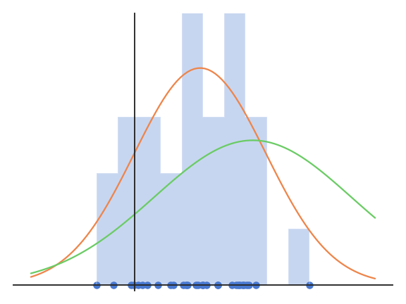
Fig. 4.8 Normal distributions with different parameters \(\mu\) and \(\sigma\) explain the data with different likelihoods.

The problem is to find the values of \(\mu\) and \(\sigma\) which explain best the observations \(\{x_i\}_{i=1}^N\).

The idea of MLE is to maximize the joint density function for all observations. This function is expressed by the likelihood function:

\[ L(\mu, \sigma) = P( x ; \mu , \sigma ) = \prod_{i=1}^{N} f(x_i ; \mu, \sigma ) \]

When the pdf takes high values for all samples, it is quite likely that the samples come from this particular distribution. The likelihood function reflects the probability that the parameters \(\mu\) and \(\sigma\) explain the observations \(\{x_i\}_{i=1}^N\).

We therefore search for the values \(\mu\) and \(\sigma\) which maximize the likelihood function.

\[ \text{max}_{\mu, \sigma} \quad L(\mu, \sigma) = \prod_{i=1}^{N} f(x_i ; \mu, \sigma ) \]

For the normal distribution, the likelihood function is:

\[\begin{split} \begin{aligned} L(\mu, \sigma) & = \prod_{i=1}^{N} f(x_i ; \mu, \sigma ) \\ & = \prod_{i=1}^{N} \frac{1}{\sqrt{2\pi \sigma^2}} \, \exp{- \frac{(x_i - \mu)^2}{2\sigma^2}}\\ & = (\frac{1}{\sqrt{2\pi \sigma^2}})^N \, \prod_{i=1}^{N} \exp{- \frac{(x_i - \mu)^2}{2\sigma^2}}\\ & = (\frac{1}{\sqrt{2\pi \sigma^2}})^N \, \exp{- \frac{\sum_{i=1}^{N}(x_i - \mu)^2}{2\sigma^2}}\\ \end{aligned} \end{split}\]

To find the maximum of \(L(\mu, \sigma)\), we need to search where the gradient is equal to zero:

\[\begin{split} \begin{cases} \dfrac{\partial L(\mu, \sigma)}{\partial \mu} = 0 \\ \dfrac{\partial L(\mu, \sigma)}{\partial \sigma} = 0 \\ \end{cases} \end{split}\]

The likelihood function is complex to differentiate, so we consider its logarithm \(l(\mu, \sigma) = \log(L(\mu, \sigma))\) which has a maximum for the same value of \((\mu, \sigma)\) as the log function is monotonic.

\[\begin{split} \begin{aligned} l(\mu, \sigma) & = \log(L(\mu, \sigma)) \\ & = \log \left((\frac{1}{\sqrt{2\pi \sigma^2}})^N \, \exp{- \frac{\sum_{i=1}^{N}(x_i - \mu)^2}{2\sigma^2}} \right)\\ & = - \frac{N}{2} \log (2\pi \sigma^2) - \frac{\sum_{i=1}^{N}(x_i - \mu)^2}{2\sigma^2}\\ \end{aligned} \end{split}\]

\(l(\mu, \sigma)\) is called the log-likelihood function. The maximum of the log-likelihood function respects:

\[\begin{split} \begin{aligned} \frac{\partial l(\mu, \sigma)}{\partial \mu} & = \frac{\sum_{i=1}^{N}(x_i - \mu)}{\sigma^2} = 0 \\ \frac{\partial l(\mu, \sigma)}{\partial \sigma} & = - \frac{N}{2} \frac{4 \pi \sigma}{2 \pi \sigma^2} + \frac{\sum_{i=1}^{N}(x_i - \mu)^2}{\sigma^3} \\ & = - \frac{N}{\sigma} + \frac{\sum_{i=1}^{N}(x_i - \mu)^2}{\sigma^3} = 0\\ \end{aligned} \end{split}\]

We obtain:

\[ \mu = \frac{1}{N} \sum_{i=1}^{N} x_i \qquad\qquad \sigma^2 = \frac{1}{N} \sum_{i=1}^{N}(x_i - \mu)^2 \]

Unsurprisingly, the mean and variance of the normal distribution which best explains the data are the mean and variance of the data…

The same principle can be applied to estimate the parameters of any distribution: normal, exponential, Bernouilli, Poisson, etc… When a machine learning method has an probabilistic interpretation (i.e. it outputs probabilities), MLE can be used to find its parameters. One can use global optimization like here, or gradient descent to estimate the parameters iteratively.

4.3. Soft linear classification : Logistic regression

In logistic regression, we want to perform a regression, but where the targets \(t_i\) are bounded betwen 0 and 1. We can use a logistic function instead of a linear function in order to transform the net activation into an output:

\[ \begin{aligned} y = \sigma(w \, x + b ) = \frac{1}{1+\exp(-w \, x - b )} \end{aligned} \]

Logistic regression can be used in binary classification if we consider \(y = \sigma(w \, x + b )\) as the probability that the example belongs to the positive class (\(t=1\)).

\[ P(t = 1 | x; w, b) = y ; \qquad P(t = 0 | x; w, b) = 1 - y \]

The output \(t\) therefore comes from a Bernouilli distribution \(\mathcal{B}\) of parameter \(p = y = f_{w, b}(x)\). The probability density function (pdf) is:

\[f(t | x; w, b) = y^t \, (1- y)^{1-t}\]

If we consider our training samples \((x_i, t_i)\) as independently taken from this distribution, our task is to find the parameterized distribution that best explains the data, which means to find the parameters \(w\) and \(b\) maximizing the likelihood that the samples \(t\) come from a Bernouilli distribution when \(x\), \(w\) and \(b\) are given. We only need to apply Maximum Likelihood Estimation (MLE) on this Bernouilli distribution!

The likelihood function for logistic regression is :

\[\begin{split} \begin{aligned} L( w, b) &= P( t | x; w, b ) = \prod_{i=1}^{N} f(t_i | x_i; w, b ) \\ &= \prod_{i=1}^{N} y_i^{t_i} \, (1- y_i)^{1-t_i} \end{aligned} \end{split}\]

The likelihood function is quite hard to differentiate, so we take the log-likelihood function:

\[\begin{split} \begin{aligned} l( w, b) &= \log L( w, b) \\ &= \sum_{i=1}^{N} [t_i \, \log y_i + (1 - t_i) \, \log( 1- y_i)]\\ \end{aligned} \end{split}\]

or even better: the negative log-likelihood which will be minimized using gradient descent:

\[ \mathcal{L}( w, b) = - \sum_{i=1}^{N} [t_i \, \log y_i + (1 - t_i) \, \log( 1- y_i)] \]

We then search for the minimum of the negative log-likelihood function by computing its gradient (here for a single sample):

\[\begin{split} \begin{aligned} \frac{\partial \mathcal{l}_i(w, b)}{\partial w} &= -\frac{\partial}{\partial w} [ t_i \, \log y_i + (1 - t_i) \, \log( 1- y_i) ] \\ &= - t_i \, \frac{\partial}{\partial w} \log y_i - (1 - t_i) \, \frac{\partial}{\partial w}\log( 1- y_i) \\ &= - t_i \, \frac{\frac{\partial}{\partial w} y_i}{y_i} - (1 - t_i) \, \frac{\frac{\partial}{\partial w}( 1- y_i)}{1- y_i} \\ &= - t_i \, \frac{y_i \, (1 - y_i) \, x_i}{y_i} + (1 - t_i) \, \frac{y_i \, (1-y_i) \, x_i}{1 - y_i}\\ &= - ( t_i - y_i ) \, x_i\\ \end{aligned} \end{split}\]

We obtain the same gradient as the linear perceptron, but with a non-linear output function! Logistic regression is therefore a regression method used for classification. It uses a non-linear transfer function \(\sigma(x)=\frac{1}{1+\exp(-x)}\) applied on the net activation:

\[ y_i = \sigma(\langle \mathbf{w} \cdot \mathbf{x}_i \rangle + b ) \]

The continuous output \(y\) is interpreted as the probability of belonging to the positive class.

\[ P(t_i = 1 | \mathbf{x}_i; \mathbf{w}, b) = y_i ; \qquad P(t_i = 0 | \mathbf{x}_i; \mathbf{w}, b) = 1 - y_i \]

We minimize the negative log-likelihood loss function:

\[ \mathcal{L}(\mathbf{w}, b) = - \sum_{i=1}^{N} [t_i \, \log y_i + (1 - t_i) \, \log( 1- y_i)] \]

Gradient descent leads to the delta learning rule, using the class as a target and the probability as a prediction:

\[\begin{split} \begin{cases} \Delta \mathbf{w} = \eta \, ( t_i - y_i ) \, \mathbf{x}_i \\ \\ \Delta b = \eta \, ( t_i - y_i ) \\ \end{cases} \end{split}\]

Logistic regression

• \(\mathbf{w} = 0 \qquad b = 0\)

• for \(M\) epochs:

  • for each sample \((\mathbf{x}_i, t_i)\):

    • \(y_i = \sigma( \langle \mathbf{w} \cdot \mathbf{x}_i \rangle + b)\)

    • \(\Delta \mathbf{w} = \eta \, (t_i - y_i) \, \mathbf{x}_i\)

    • \(\Delta b = \eta \, (t_i - y_i)\)

Logistic regression works just like linear classification, except in the way the prediction is done. To know to which class \(\mathbf{x}_i\) belongs, simply draw a random number between 0 and 1:

• if it is smaller than \(y_i\) (probability \(y_i\)), it belongs to the positive class.

• if it is bigger than \(y_i\) (probability \(1-y_i\)), it belongs to the negative class.

Alternatively, you can put a hard limit at 0.5:

• if \(y_i > 0.5\) then the class is positive.

• if \(y_i < 0.5\) then the class is negative.

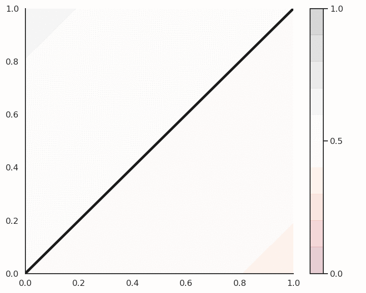
Fig. 4.9 Logistic regression for soft classification. The confidence scores tells how certain the classification is.

Logistic regression also provides a confidence score: the closer \(y\) is from 0 or 1, the more confident we can be that the classification is correct. This is particularly important in safety critical applications: if you detect the positive class but with a confidence of 0.51, you should perhaps not trust the prediction. If the confidence score is 0.99, you can probably trust the prediction.

previous

3. Regularization

next

5. Multi-class classification