.md .pdf

Contents

5. Spiking neural networks

Slides: pdf

5.1. Spiking neurons

5.1.1. Spiking neuron models

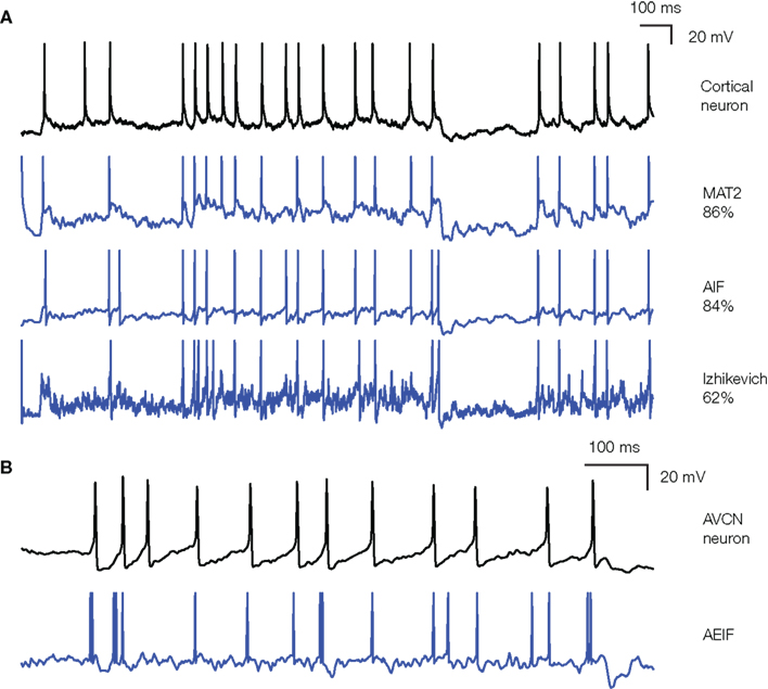
Fig. 5.21 Spike trains. Source: [Rossant et al., 2011].

The two important dimensions of the information exchanged by neurons are:

1. The instantaneous frequency or firing rate: number of spikes per second (Hz).

2. The precise timing of the spikes.

The shape of the spike (amplitude, duration) does not matter much. Spikes are binary signals (0 or 1) at precise moments of time. Rate-coded neurons only represent the firing rate of a neuron and ignore spike timing. Spiking neurons represent explicitly spike timing, but omit the details of action potentials.

The leaky integrate-and-fire (LIF; Lapicque, 1907) neuron has a membrane potential \(v(t)\) that integrates its input current \(I(t)\):

\[ C \, \frac{dv(t)}{dt} = - g_L \, (v(t) - V_L) + I(t) \]

\(C\) is the membrane capacitance, \(g_L\) the leak conductance and \(V_L\) the resting potential. In the absence of input current (\(I=0\)), the membrane potential is equal to the resting potential.

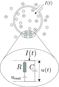
Fig. 5.22 Membrane potential of a leaky integrate-and-fire neuron. Source: https://neuronaldynamics.epfl.ch/online/Ch1.S3.html.

When the membrane potential exceeds a threshold \(V_T\), the neuron emits a spike and the membrane potential is reset to the reset potential \(V_r\) for a fixed refractory period \(t_\text{ref}\).

\[ \text{if} \; v(t) > V_T \; \text{: emit a spike and set} \, v(t) = V_r \; \text{for} \, t_\text{ref} \, \text{ms.} \]

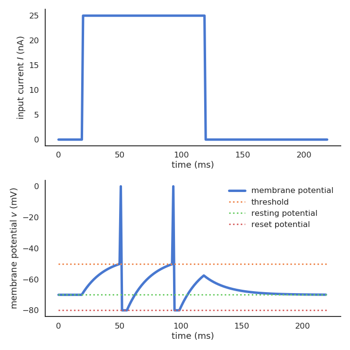
Fig. 5.23 Spike emission of a leaky integrate-and-fire neuron.

Different spiking neuron models are possible:

• Izhikevich quadratic IF [Izhikevich, 2003].

\[ \frac{dv(t)}{dt} = 0.04 \, v(t)^2 + 5 \, v(t) + 140 - u(t) + I(t) \]

\[ \frac{du(t)}{dt} = a \, (b \, v(t) - u(t)) \]

• Adaptive exponential IF (AdEx, [Brette & Gerstner, 2005]).

\[ C \, \frac{dv(t)}{dt} = -g_L \ (v(t) - E_L) + g_L \, \Delta_T \, \exp(\frac{v(t) - v_T}{\Delta_T}) + I(t) - w \]

\[ \tau_w \, \frac{dw}{dt} = a \, (v(t) - E_L) - w \]

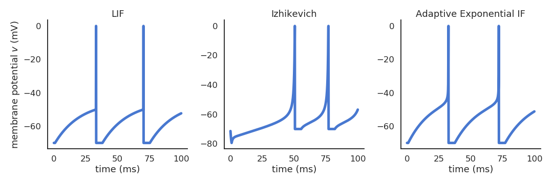
Fig. 5.24 LIF, Izhikevich and AdEx neurons.

Biological neurons do not all respond the same to an input current.

• Some fire regularly.

• Some slow down with time.

• Some emit bursts of spikes.

Modern spiking neuron models allow to recreate these dynamics by changing a few parameters.

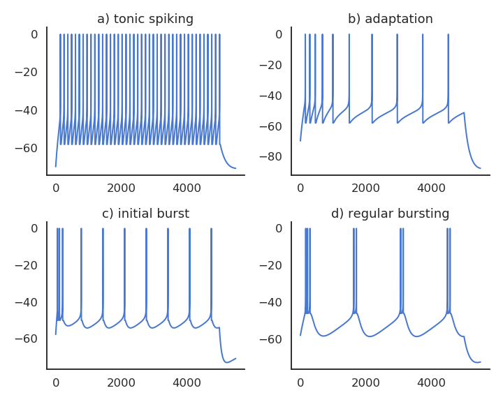
Fig. 5.25 Variety of neural dynamics.

5.1.2. Synaptic transmission

Spiking neurons communicate by increasing the conductance \(g_e\) of the postsynaptic neuron:

\[ C \, \frac{dv(t)}{dt} = - g_L \, (v(t) - V_L) - g_e(t) \, (v(t) - V_E) + I(t) \]

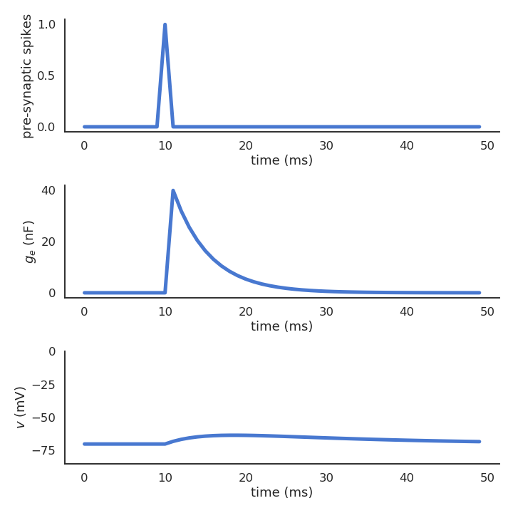
Fig. 5.26 Synaptic transmission for a single incoming spike.

Incoming spikes increase the conductance from a constant \(w\) which represents the synaptic efficiency (or weight):

\[ g_e(t) \leftarrow g_e(t) + w \]

If there is no spike, the conductance decays back to zero:

\[ \tau_e \, \frac{d g_e(t)}{dt} + g_e(t) = 0 \]

An incoming spike temporarily increases (or decreases if the weight \(w\) is negative) the membrane potential of the post-synaptic neuron.

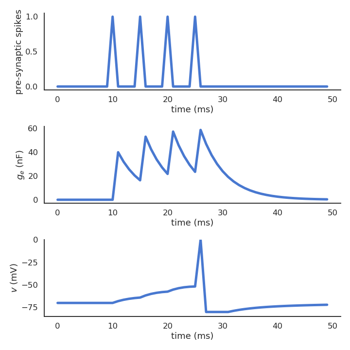
Fig. 5.27 Synaptic transmission for multiple incoming spikes.

When enough spikes arrive at the post-synaptic neuron close in time:

• either one pre-synaptic fires very rapidly,

• or many different pre-synaptic neurons fire in close proximity, this can be enough to bring the post-synaptic membrane over the threshold, so that it it turns emits a spike. This is the basic principle of synaptic transmission in biological neurons. Neurons emit spikes, which modify the membrane potential of other neurons, which in turn emit spikes, and so on.

5.1.3. Populations of spiking neurons

Recurrent networks of spiking neurons exhibit various dynamics. They can fire randomly, or tend to fire synchronously, depending on their inputs and the strength of the connections. Liquid State Machines are the spiking equivalent of echo-state networks.

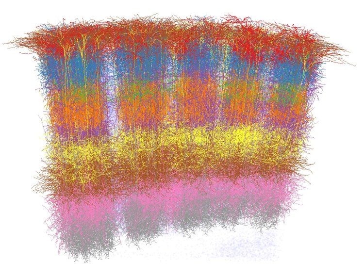
Fig. 5.28 Cortical column of the rat’s vibrissal cortex. Source: https://www.pnas.org/content/110/47/19113.

5.1.4. Synaptic plasticity

Hebbian learning postulates that synapses strengthen based on the correlation between the activity of the pre- and post-synaptic neurons:

When an axon of cell A is near enough to excite a cell B and repeatedly or persistently takes part in firing it, some growth process or metabolic change takes place in one or both cells such that A’s efficiency, as one of the cells firing B, is increased.

Donald Hebb, 1949

Synaptic efficiencies actually evolve depending on the the causation between the neuron’s firing patterns:

• If the pre-synaptic neuron fires before the post-synaptic one, the weight is increased (long-term potentiation). Pre causes Post to fire.

• If it fires after, the weight is decreased (long-term depression). Pre does not cause Post to fire.

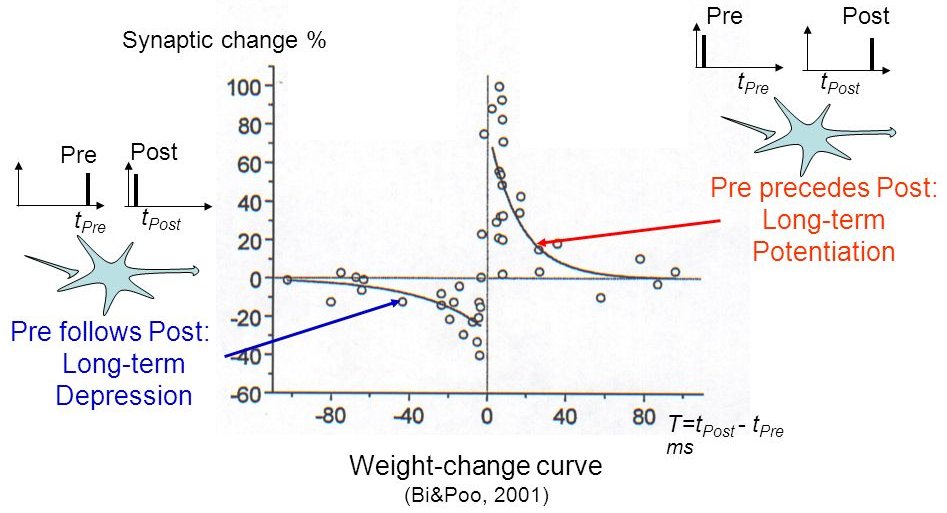
Fig. 5.29 Spike-timing dependent plasticity. Source: [Bi & Poo, 2001].

The STDP (spike-timing dependent plasticity) plasticity rule describes how the weight of a synapse evolves when the pre-synaptic neuron fires at \(t_\text{pre}\) and the post-synaptic one fires at \(t_\text{post}\).

\[\begin{split} \Delta w = \begin{cases} A^+ \, \exp - \frac{t_\text{pre} - t_\text{post}}{\tau^+} \; \text{if} \; t_\text{post} > t_\text{pre}\\ A^- \, \exp - \frac{t_\text{pre} - t_\text{post}}{\tau^-} \; \text{if} \; t_\text{pre} > t_\text{post}\\ \end{cases}\end{split}\]

STDP can be implemented online using traces. More complex variants of STDP (triplet STDP) exist, but this is the main model of synaptic plasticity in spiking networks.

5.2. Deep convolutional spiking networks

A lot of work has lately focused on deep spiking networks, either using a modified version of backpropagation or using STDP. The Masquelier lab [Kheradpisheh et al., 2018] has proposed a deep spiking convolutional network learning to extract features using STDP (unsupervised learning). A simple classifier (SVM) then learns to predict classes.

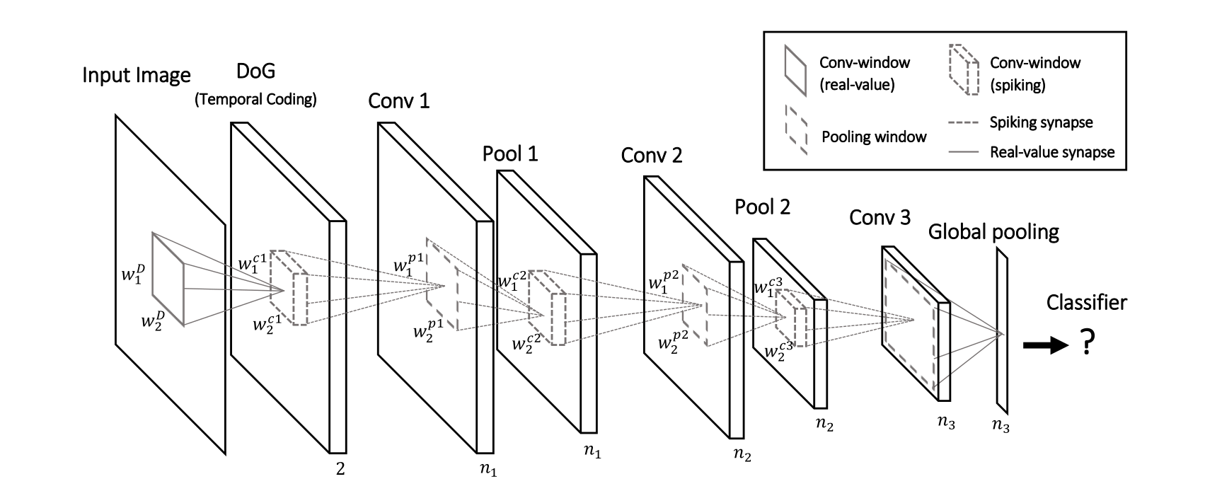
Fig. 5.30 Deep convolutional spiking network of [Kheradpisheh et al., 2018].

The image is first transformed into a spiking population using difference-of-Gaussian (DoG) filters.

• On-center neurons fire when a bright area at the corresponding location is surrounded by a darker area.

• Off-center cells do the opposite.

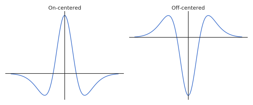
Fig. 5.31 Preprocessing using DoG filters.

The convolutional and pooling layers work just as in regular CNNs (shared weights), except the neuron are integrate-and-fire (IF). There is additionally a temporal coding scheme, where the first neuron to emit a spike at a particular location (i.e. over all feature maps) inhibits all the others. This ensures selectivity of the features through sparse coding: only one feature can be detected at a given location. STDP allows to learn causation between the features and to extract increasingly complex features.

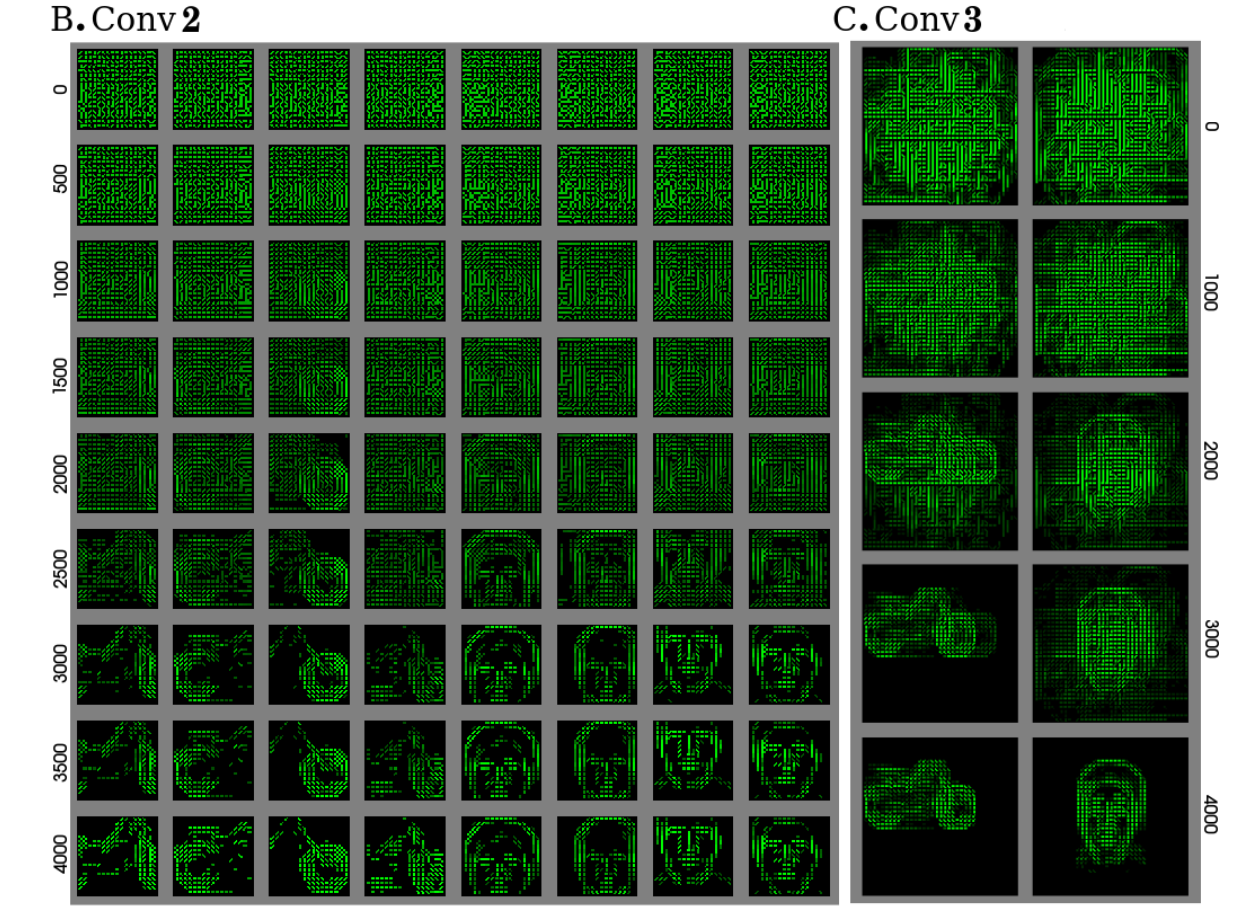
Fig. 5.32 Spiking activity in the convolutional layers. Source: [Kheradpisheh et al., 2018].

The network is trained unsupervisedly on various datasets and obtains accuracies close to the state of the art (Caltech face/motorbike dataset, ETH-80, MNIST)

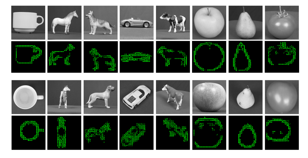
Fig. 5.33 Activity in the model for different images. Source: [Kheradpisheh et al., 2018].

The performance on MNIST is in line with classical 3-layered CNNs, but without backpropagation!

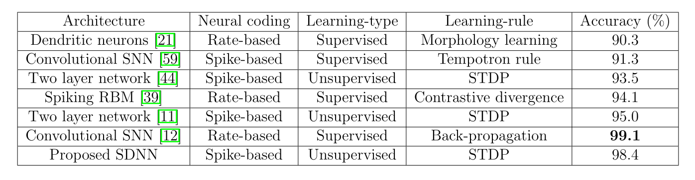
Fig. 5.34 The spiking network achieves 98.4% accuracy on MNIST fully unsupervised. Source: [Kheradpisheh et al., 2018].

5.3. Neuromorphic computing

5.3.1. Event-based cameras

Event-based cameras are inspired from the retina (neuromorphic) and emit spikes corresponding to luminosity changes. Classical computers cannot cope with the high fps of event-based cameras. Spiking neural networks can be used to process the events (classification, control, etc). But do we have the hardware for that?

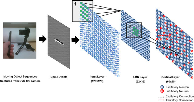
Fig. 5.35 Event-based cameras can be used as inputs to spiking networks. Source: https://www.researchgate.net/publication/280600732_A_Computational_Model_of_Innate_Directional_Selectivity_Refined_by_Visual_Experience

5.3.2. Intel Loihi

Intel Loihi is a neuromorphic chip that implements 128 neuromorphic cores, each containing 1,024 primitive spiking neural units grouped into tree-like structures in order to simplify the implementation.

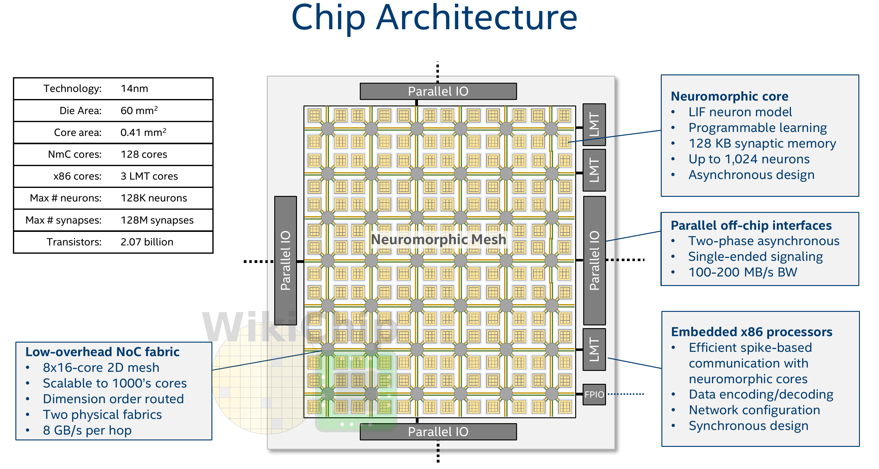
Fig. 5.36 Architecture of Intel Loihi. Source: https://en.wikichip.org/wiki/intel/loihi

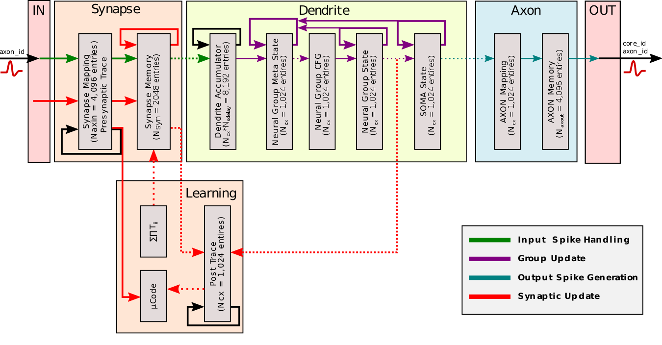
Fig. 5.37 Architecture of Intel Loihi. Source: https://en.wikichip.org/wiki/intel/loihi

Fig. 5.38 Spike propagation in Intel Loihi. Source: https://en.wikichip.org/wiki/intel/loihi

Each neuromorphic core transits spikes to the other cores. Fortunately, the firing rates are usually low (10 Hz), what limits the communication costs inside the chip. Synapses are learnable with STDP mechanisms (memristors), although offline.

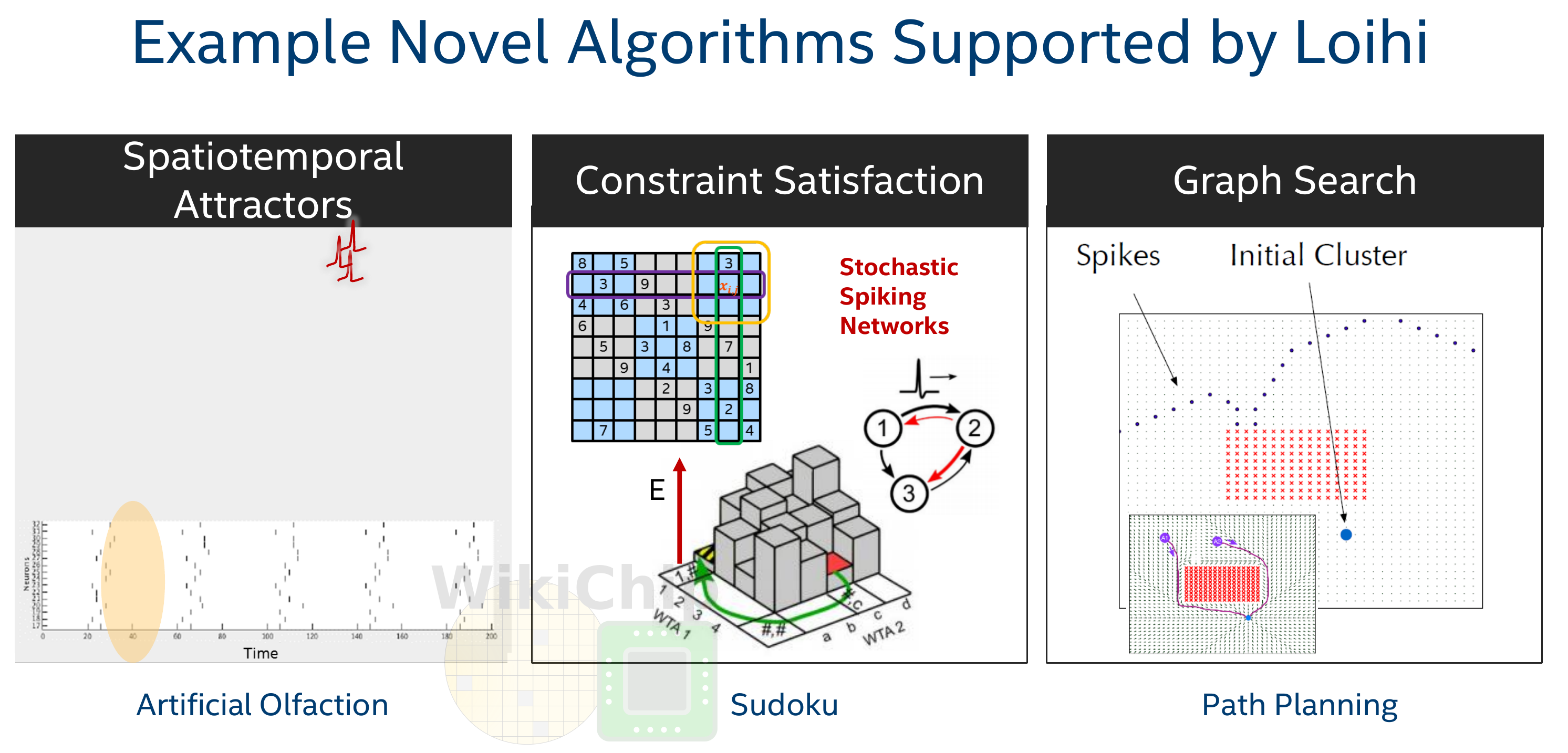
Fig. 5.39 Intel Loihi allows to implement various ML algorithms. Source: https://en.wikichip.org/wiki/intel/loihi

Intel Loihi consumes 1/1000th of the energy needed by a modern GPU. Alternatives to Intel Loihi are:

• IBM TrueNorth

• Spinnaker (University of Manchester).

• Brainchip

The number of simulated neurons and synapses is still very far away from the human brain, but getting closer!

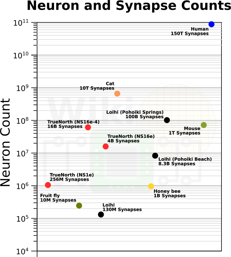
Fig. 5.40 Number of neurons and synapses in various neuromorphic architectures. Source: https://fuse.wikichip.org/news/2519/intel-labs-builds-a-neuromorphic-system-with-64-to-768-loihi-chips-8-million-to-100-million-neurons/

5.3.3. Towards biologically inspired AI

Next-gen AI should overcome the limitations of deep learning by:

• Making use of unsupervised learning rules (Hebbian, STDP).

• Using neural and population dynamics (reservoir) to decompose inputs into a spatio-temporal space, instead of purely spatial.

• Use energy-efficient neural models (spiking neurons) able to run efficiently on neuromorphic hardware.

• Design more complex architectures and use embodiment.

previous

4. Unsupervised Hebbian learning

next

1. Introduction to Python