.md .pdf

Contents

3. Regularization

Slides: pdf

3.1. A bit of learning theory

Before going further, let’s think about what we have been doing so far. We had a bunch of data samples \(\mathcal{D} = (\mathbf{x}_i, t_i)_{i=1..N}\) (the training set). We decided to apply a (linear) model on it:

\[y_i = \langle \mathbf{w} . \mathbf{x}_i \rangle + b\]

We then minimized the mean square error (mse) on that training set using gradient descent:

\[ \mathcal{L}(w, b) = \mathbb{E}_{\mathbf{x}, t \in \mathcal{D}} [(t_i - y_i )^2] \]

At the end of learning, we can measure the residual error of the model on the data:

\[ \epsilon_\mathcal{D} = \frac{1}{N} \, \sum_{i=1}^{N} (t_i - y_i )^2 \]

We get a number, for example 0.04567. Is that good?

The mean square error mse is not very informative, as its value depends on how the outputs are scaled: multiply the targets and prediction by 10 and the mse is 100 times higher.

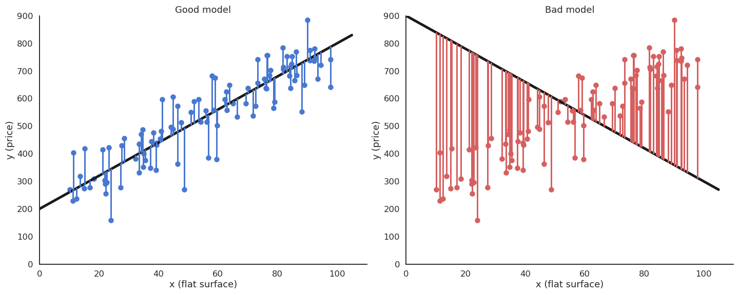
Fig. 3.21 The residual error measures the quality of the fit, but it is sensible to the scaling of the outputs.

The coefficient of determination \(R^2\) is a rescaled variant of the mse comparing the variance of the residuals to the variance of the data around its mean \(\hat{t}\):

\[ R^2 = 1 - \frac{\text{Var}(\text{residuals})}{\text{Var}(\text{data})} = 1 - \frac{\sum_{i=1}^N (t_i- y_i)^2}{\sum_{i=1}^N (t_i - \hat{t})^2} \]

\(R^2\) should be as close from 1 as possible. For example, if \(R^2 = 0.8\), we can say that the model explains 80% of the variance of the data.

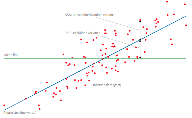
Fig. 3.22 The coefficient of determination compares the variance of the residuals to the variance of the data. Source: https://towardsdatascience.com/introduction-to-linear-regression-in-python-c12a072bedf0

3.1.1. Sensibility to outliers

Suppose we have a training set with one outlier (bad measurement, bad luck, etc).

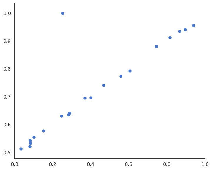
Fig. 3.23 Linear data with one outlier.

LMS would find the minimum of the mse, but it is clearly a bad fit for most points.

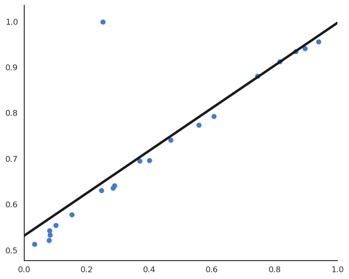
Fig. 3.24 LMS is attracted by the outlier, leading to a bad prediction for all points.

This model feels much better, but its residual mse is actually higher…

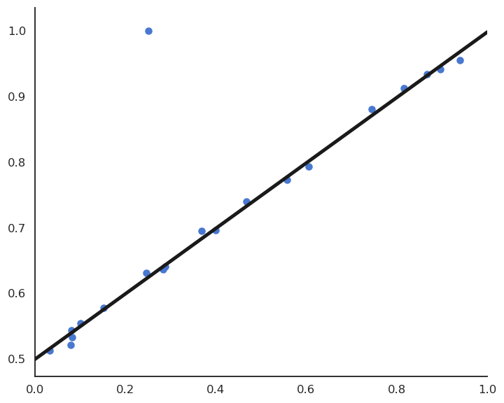
Fig. 3.25 By ignoring the outlier, the prediction would be correct for most points.

Let’s visualize polynomial regression with various orders of the polynomial on a small dataset.

Fig. 3.26 Polynomial regression with various orders.

When only looking at the residual mse on the training data, one could think that the higher the order of the polynomial, the better. But it is obvious that the interpolation quickly becomes very bad when the order is too high. A complex model (with a lot of parameters) is useless for predicting new values. We actually do not care about the error on the training set, but about generalization.

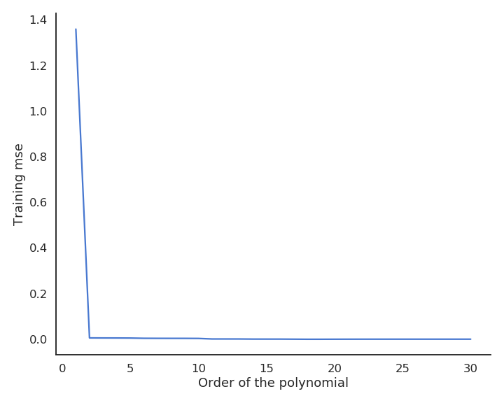
Fig. 3.27 Residual mse of polynomial regression depending on the order of the polynomial.

3.1.2. Cross-validation

Let’s suppose we dispose of \(m\) models \(\mathcal{M} = \{ M_1, ..., M_m\}\) that could be used to fit (or classify) some data \(\mathcal{D} = \{\mathbf{x}_i, t_i\}_{i=1}^N\). Such a class could be the ensemble of polynomes with different orders, different algorithms (NN, SVM) or the same algorithm with different values for the hyperparameters (learning rate, regularization parameters…).

The naive and wrong method to find the best hypothesis would be:

Do not do this!

• For all models \(M_i\):

  • Train \(M_i\) on \(\mathcal{D}\) to obtain an hypothesis \(h_i\).

  • Compute the training error \(\epsilon_\mathcal{D}(h_i)\) of \(h_i\) on \(\mathcal{D}\) :

  \[ \epsilon_\mathcal{D}(h_i) = \mathbb{E}_{(\mathbf{x}, t) \in \mathcal{D}} [(h_i(\mathbf{x}) - t)^2] \]

• Select the hypothesis \(h_{i}^*\) with the minimal training error : \(h_{i}^* = \text{argmin}_{h_i \in \mathcal{M}} \quad \epsilon_\mathcal{D}(h_i)\)

This method leads to overfitting, as only the training error is used.

The solution is randomly take some samples out of the training set to form the test set. Typical values are 20 or 30 % of the samples in the test set.

1. Train the model on the training set (70% of the data).

2. Test the performance of the model on the test set (30% of the data).

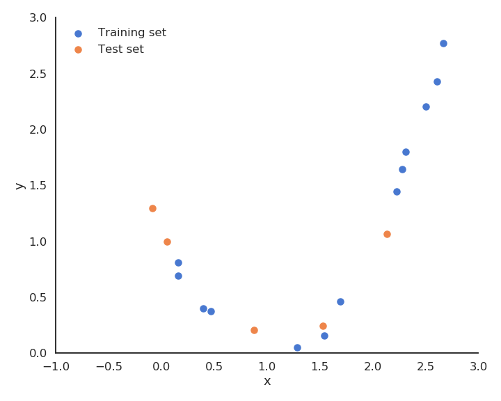
Fig. 3.28 Polynomial data split in a training set and a test set.

The test performance will better measure how well the model generalizes to new examples.

Simple hold-out cross-validation

• Split the training data \(\mathcal{D}\) into \(\mathcal{S}_{\text{train}}\) and \(\mathcal{S}_{\text{test}}\).

• For all models \(M_i\):

  • Train \(M_i\) on \(\mathcal{S}_{\text{train}}\) to obtain an hypothesis \(h_i\).

  • Compute the empirical error \(\epsilon_{\text{test}}(h_i)\) of \(h_i\) on \(\mathcal{S}_{\text{test}}\) :

  \[\epsilon_{\text{test}}(h_i) = \mathbb{E}_{(\mathbf{x}, t) \in \mathcal{S}_{\text{test}}} [(h_i(\mathbf{x}) - t)^2]\]

• Select the hypothesis \(h_{i}^*\) with the minimal empirical error : \(h_{i}^* = \text{argmin}_{h_i \in \mathcal{M}} \quad \epsilon_{\text{test}}(h_i)\)

The disadvantage of simple hold-out cross-validation is that 20 or 30% of the data is wasted and not used for learning. It may be a problem when data is rare or expensive.

k-fold cross-validation allows a more efficient use os the available data and a better measure of the generalization error. The idea is to build several different training/test sets with the same data, train and test each model repeatedly on each partition and choose the hypothesis that works best on average.

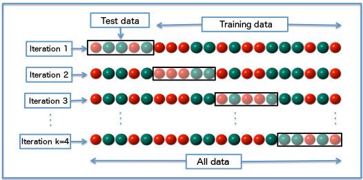
Fig. 3.29 k-fold cross-validation. Source https://upload.wikimedia.org/wikipedia/commons/1/1c/K-fold_cross_validation_EN.jpg

k-fold cross-validation

• Randomly split the data \(\mathcal{D}\) into \(k\) subsets of \(\frac{N}{k}\) examples \(\{ \mathcal{S}_{1}, \dots , \mathcal{S}_{k}\}\)

• For all models \(M_i\):

  • For all \(k\) subsets \(\mathcal{S}_j\):

    • Train \(M_i\) on \(\mathcal{D} - \mathcal{S}_j\) to obtain an hypothesis \(h_{ij}\)

    • Compute the empirical error \(\epsilon_{\mathcal{S}_j}(h_{ij})\) of \(h_{ij}\) on \(\mathcal{S}_j\)

  • The empirical error of the model \(M_i\) on \(\mathcal{D}\) is the average of empirical errors made on \((\mathcal{S}_j)_{j=1}^{k}\)

    \[ \epsilon_{\mathcal{D}} (M_i) = \frac{1}{k} \cdot \sum_{j=1}^{k} \epsilon_{\mathcal{S}_j}(h_{ij}) \]

• Select the model \(M_{i}^*\) with the minimal empirical error on \(\mathcal{D}\).

In general, you can take \(k=10\) partitions. The extreme case is to take \(k=N\) partition, i.e. the test set has only one sample each time: leave-one-out cross-validation. k-fold cross-validation works well, but needs a lot of repeated learning.

3.1.3. Underfitting - overfitting

While the training mse always decrease with more complex models, the test mse increases after a while. This is called overfitting: learning by heart the data without caring about generalization. The two curves suggest that we should chose a polynomial order between 2 and 9.

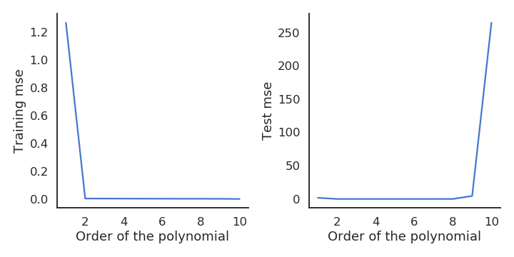
Fig. 3.30 Training and test mse of polynomial regression.

A model not complex enough for the data will underfit: its training error is high. A model too complex for the data will overfit: its test error is high. In between, there is the right complexity for the model: it learns the data correctly but does not overfit.

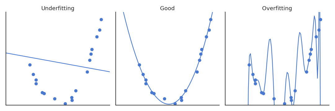
Fig. 3.31 Underfitting and overfitting.

What does complexity mean? In polynomial regression, the complexity is related to the order of the polynomial, i.e. the number of coefficients to estimate:

\[y = f_{\mathbf{w}, b}(x) = \sum_{k=1}^p w_k \, x^k + b\]

\[\begin{split}\mathbf{x} = \begin{bmatrix} x \\ x^2 \\ \ldots \\ x^p \end{bmatrix} \qquad \mathbf{w} = \begin{bmatrix} w_1 \\ w_2 \\ \ldots \\ w_p \end{bmatrix}\end{split}\]

A polynomial of order \(p\) has \(p+1\) unknown parameters (free parameters): the \(p\) weights and the bias. Generally, the complexity of a model relates to its number of free parameters:

The more free parameters, the more complex the model is, the more likely it will overfit.

Under-/Over-fitting relates to the statistical concept of bias-variance trade-off. The bias is the training error that the hypothesis would make if the training set was infinite (accuracy, flexibility of the model): a model with high bias is underfitting. The variance is the error that will be made by the hypothesis on new examples taken from the same distribution (spread, the model is correct on average, but not for individual samples): a model with high variance is overfitting.

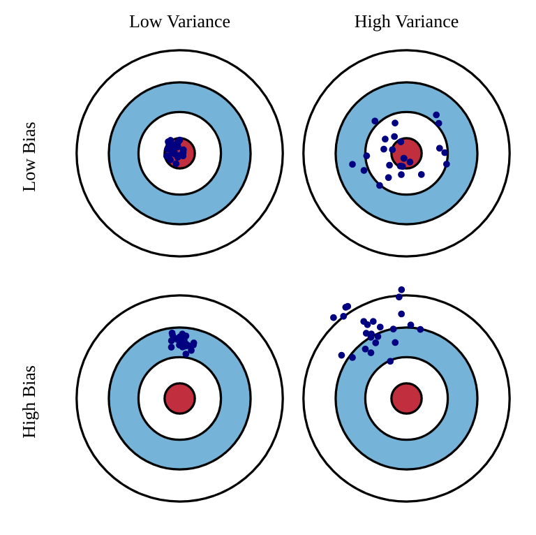
Fig. 3.32 Bias and variance of an estimator. Source: http://scott.fortmann-roe.com/docs/BiasVariance.html

The bias decreases when the model becomes complex; the variance increases when the model becomes complex. The generalization error is a combination of the bias and variance:

\[ \text{generalization error} = \text{bias}^2 + \text{variance} \]

We search for the model with the optimum complexity realizing the trade-off between bias and variance. It is better to have a model with a slightly higher bias (training error) but with a smaller variance (generalization error).

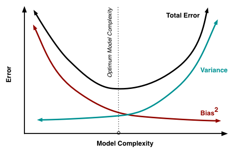
Fig. 3.33 The optimal complexity of an algorithm is a trade-off between bias and variance. Source: http://scott.fortmann-roe.com/docs/BiasVariance.html

3.2. Regularized regression

Linear regression can either underfit or overfit depending on the data.

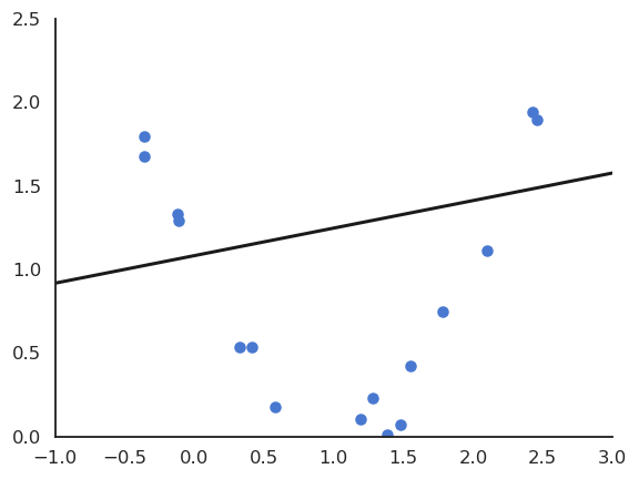
Fig. 3.34 Linear regression underfits non-linear data.

Fig. 3.35 Linear regression overfits outliers.

When linear regression underfits (both training and test errors are high), the data is not linear: we need to use a neural network. When linear regression overfits (the test error is higher than the training error), we would like to decrease its complexity.

The problem is that the number of free parameters in linear regression only depends on the number of inputs (dimensions of the input space).

\[ y = \sum_{i=1}^d w_i \, x_i + b \]

For \(d\) inputs, there are \(d+1\) free parameters: the \(d\) weights and the bias.

We must find a way to reduce the complexity of the linear regression without changing the number of parameters, which is impossible. The solution is to constrain the values that the parameters can take: regularization. Regularization reduces the variance at the cost of increasing the bias.

3.2.1. L2 regularization - Ridge regression

Using L2 regularization for linear regression leads to the Ridge regression algorithm. The individual loss function is defined as:

\[ \mathcal{l}_i(\mathbf{w}, b) = (t_i - y_i)^2 + \lambda \, ||\mathbf{w}||^2 \]

The first part of the loss function is the classical mse on the training set: its role is to reduce the bias. The second part minimizes the L2 norm of the weight vector (or matrix), reducing the variance:

\[ ||\mathbf{w}||^2 = \sum_{i=1}^d w_i^2 \]

Deriving the regularized delta learning rule is straightforward:

\[ \Delta w_i = \eta \, ((t_i - y_i) \ x_i - \lambda \, w_i) \]

Ridge regression is also called weight decay: even if there is no error, all weights will decay to 0.

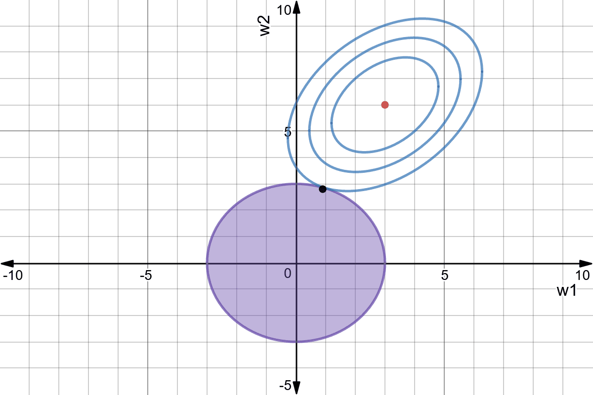
Fig. 3.36 Ridge regression finds the smallest value for the weights that minimize the mse. Source: https://www.mlalgorithms.org/articles/l1-l2-regression/

3.2.2. L1 regularization - LASSO regression

Using L1 regularization for linear regression leads to the LASSO regression algorithm (least absolute shrinkage and selection operator). The individual loss function is defined as:

\[ \mathcal{l}_i(\mathbf{w}, b) = (t_i - y_i)^2 + \lambda \, |\mathbf{w}| \]

The second part minimizes this time the L1 norm of the weight vector, i.e. its absolute value:

\[ |\mathbf{w}| = \sum_{i=1}^d |w_i| \]

Regularized delta learning rule with LASSO:

\[ \Delta w_i = \eta \, ((t_i - y_i) \ x_i - \lambda \, \text{sign}(w_i)) \]

Weight decay does not depend on the value of the weight, only its sign. Weights can decay very fast to 0.

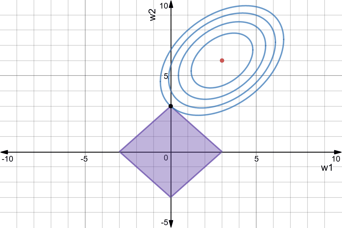
Fig. 3.37 LASSO regression tries to set as many weight to 0 as possible (sparse code). Source: https://www.mlalgorithms.org/articles/l1-l2-regression/

Both methods depend on the regularization parameter \(\lambda\). Its value determines how important the regularization term should. Regularization introduce a bias, as the solution found is not the minimum of the mse, but reduces the variance of the estimation, as small weights are less sensible to noise.

LASSO allows feature selection: features with a zero weight can be removed from the training set.

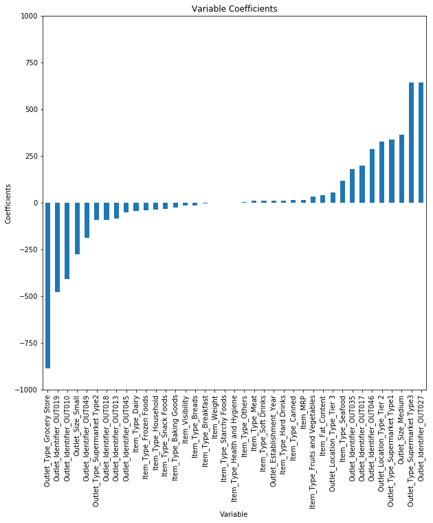
Fig. 3.38 Linear regression tends to assign values to all weights. Source: https://www.analyticsvidhya.com/blog/2017/06/a-comprehensive-guide-for-linear-ridge-and-lasso-regression/

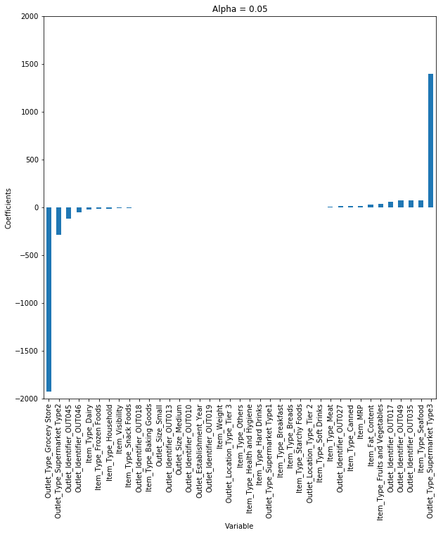
Fig. 3.39 LASSO regression tries to set as many weights to 0 as possible (sparse code). Source: https://www.analyticsvidhya.com/blog/2017/06/a-comprehensive-guide-for-linear-ridge-and-lasso-regression/

3.2.3. L1+L2 regularization - ElasticNet

An ElasticNet is a linear regression using both L1 and L2 regression:

\[ \mathcal{l}_i(\mathbf{w}, b) = (t_i - y_i)^2 + \lambda_1 \, |\mathbf{w}| + \lambda_2 \, ||\mathbf{w}||^2 \]

It combines the advantages of Ridge and LASSO, at the cost of having now two regularization parameters to determine.

previous

2. Linear Regression

next

4. Linear classification